9.2: Angular Momentum

Back in Chapter 3 we introduced the momentum of an object moving in one dimension as \(p = mv\), and found that it had the interesting property of being conserved in collisions between objects that made up an isolated system. It seems natural to ask whether the corresponding rotational quantity, formed by multiplying the “rotational inertia” \(I\) and the angular velocity \(\omega\), has any interesting properties as well. We are tentatively¹ going to call the quantity \(I\omega\) angular momentum (to distinguish it from the “ordinary,” or linear momentum, \(mv\)), and build towards a better understanding, and a formal definition of it, in the remainder of this section.

Two things are soon apparent: one is that, unlike the rotational kinetic energy, which was just plain kinetic energy, the quantity \(I\omega\) really is different from the ordinary momentum, since it has different dimensions (see the “extra” factor of \(R\) in Equation (\ref{eq:9.4}) below). The other is that there are, in fact, systems in nature where this quantity appears to remain constant to a good approximation. For instance, the Earth spinning around its axis, at a constant rate of \(2\pi\) radians every 24 hours, has, by virtue of that, a constant angular momentum (a constant \(I\) and \(\omega\)).

It is best, however, to start by thinking about how we would define “angular momentum” for a system consisting of a single particle, and then building up from there, as we have been doing all semester with every new concept. For a particle moving in a circle, according to the previous section, the moment of inertia is just \(I = mR^2\), and therefore \(I\omega\) is just \(mR^2\omega\). Using Equation (8.4.12), we can write (the letter \(L\) is the conventional symbol for angular momentum; do not mistake it for a length!)

\[ L=I \omega=\pm m R|v| \quad \mathrm{ (particle \: moving \: in \: a \: circle) } \label{eq:9.4} \]

where, for consistency with our sign convention for \(\omega\), we should use the positive sign if the rotation is counterclockwise, and the negative sign if it is clockwise.

We can again readily think of examples in nature where the quantity (\ref{eq:9.4}) is conserved: for instance, the moon, if we treat it as a particle orbiting the Earth in an approximately circular orbit², has then an approximately constant angular momentum, as given by Equation (\ref{eq:9.4}). This example is also interesting because it offers an inkling of an important difference between ordinary momentum, and angular momentum: it appears that the latter can be conserved even in the presence of some kinds of external forces (in this case, the force of gravity due to the Earth that keeps the moon on its orbit).

On the other hand, it is not immediately obvious how to generalize the definition (9.4) to other kinds of motion. If we simply try something like \(L = mvr\), where \(r\) is the distance to a fixed axis, or to a fixed point, then we find that this yields a quantity that is constantly changing, even for the simplest possible physical system, namely, a particle moving on a straight line with constant velocity. Yet, we would like to define \(L\) in such a way that it will remain constant when, in fact, nothing in the particle’s actual state of motion is changing.

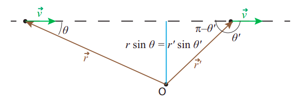
The way to do this, for a particle moving on a straight line, is to define \(L\) as the product of \(mv\) times, not the distance of the particle to a point, but the distance of the particle’s line of motion to the point considered. The “line of motion” is just a straight line that contains the velocity vector at any given time. The distance between a line and a point O is, by definition, the shortest distance from O to any point on the line; it is given by the length of a segment drawn perpendicular to the line through the point O.

For a particle moving in a circle, the line of motion at any time is tangent to the circle, and so the distance between the line of motion and the center of the circle is just the radius \(R\), so we recover the definition Equation (\ref{eq:9.4}). For the general case, on the other hand, we have the situation shown in Figure \(\PageIndex{1}\): if the instantaneous velocity of the particle is \(\vec v\), and we draw the position vector of the particle, \(\vec r\), with the point O as the origin, then the distance between O and the line of motion (sometimes also called the perpendicular distance between O and the particle) is given by \(r \sin \theta\), where \(\theta\) is the angle between the vectors \(\vec r\) and \(\vec v\).

Figure \(\PageIndex{1}\): For a particle moving on a straight line, the distance from the point O to the particle’s line of motion (dashed line) is equal to \(r \sin \theta\) at every point in the trajectory (two possible points are shown in the figure). The distance is the length of the blue segment. The figure shows there is some freedom in choosing how the angle \(\theta\) between \(\vec r\) and \(\vec v\) is to be measured, since the sine of \(\theta\) is the same as the sine of \(\pi - \theta\).

We therefore try and define angular momentum relative to a point O as the product

\[ L=\pm m r|v| \sin \theta \label{eq:9.5} \]

with the positive sign if the point O is to the left of the line of motion as the particle passes by (which corresponds to counterclockwise motion on the circle), and negative otherwise.

There are two very good things about the definition (\ref{eq:9.5}): the first one is that there is already in existence a mathematical operation between vectors, called the vector, or cross, product, according to which \(|L|\), as defined by (\ref{eq:9.5}), would just be given by \(|\vec{r} \times \vec{p}| \), where \(\vec{r} \times \vec{p} \) is the cross product of \(\vec r\) and \(\vec p\); I will have a lot more to say about this in the next subsection. The second good thing is that, with this definition, the angular momentum will be conserved in an important kind of process, namely, a collision that converts linear to rotational motion, as illustrated in Figure \(\PageIndex{2}\) below.

Figure \(\PageIndex{2}\): Collision between two particles, 1 and 2, of equal masses. Particle 2 is tied by a massless string to the point O. After the collision, particle 1 is at rest and particle 2 moves in the circle shown.

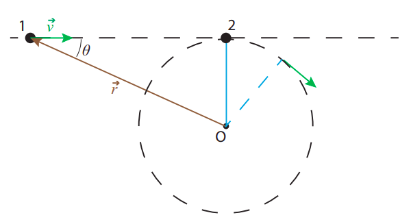
In the picture, particle 1 is initially moving with constant velocity \(\vec v\) and particle 2 is initially at rest, tied by a massless string to the point O. If the particles have the same mass, conservation of (ordinary) momentum and kinetic energy means that when they collide they exchange velocities: particle 1 comes to a stop and particle 2 starts to move to the right with the same speed v, but immediately the string starts pulling on it and bending its path into a circle. Assuming negligible friction between the string and the pivoting point (and all the surfaces involved), the speed of particle 2 will remain constant as it rotates, by conservation of kinetic energy, because the tension in the string is always perpendicular to the particle’s displacement vector, so it does no work on it.

All of the above means that angular momentum is conserved: before the collision it was equal to \(−mvr \sin \theta = −mvR\) for particle 1, and 0 for particle 2; after the collision it is zero for particle 1 and \(I\omega = mR^2\omega = −mRv\) for particle 2 (note \(\omega\) is negative, because the rotation is clockwise). Kinetic energy is also conserved, for the reasons argued above. On the other hand, ordinary momentum is only conserved until just after the collision, when the string starts pulling on particle 2, since this represents an external force on the system.

So we have found a situation in which linear motion is converted to circular motion while angular momentum, as defined by Equation (\ref{eq:9.5}), is conserved, and this despite the presence of an external force. It is true that, in fact, we were able to solve for the final motion without making explicit use of conservation of angular momentum: we only had to invoke conservation of ordinary momentum for the short duration of the collision, and conservation of kinetic energy. But it is easy to generalize the problem depicted in Figure \(\PageIndex{2}\) to one that cannot be solved by these methods, but can be solved if angular momentum is constant. Suppose that we replace particle 2 and the string by a thin rod of mass \(m\) and length \(l\) pivoted at one end. What happens now when particle 1 strikes the rod?

Figure \(\PageIndex{3}\): Collision between a particle initially moving with velocity \(\vec v_1\) and a rod of length \(l\) pivoted at an endpoint. The particle strikes the rod perpendicularly, at the other end. After the collision, the particle is moving along the same line with velocity \(\vec v_f\) , and the rod is rotating around the point O with an angular velocity \(\omega\).

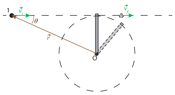
If the particle strikes the rod perpendicularly, and the collision happens very fast (that is, it is over before the rod has time to move a significant distance), we may assume the force exerted by the rod on the particle (a normal force) is along the original line of motion, so the particle will continue to move on that line. On the other hand, this time we cannot neglect the force exerted by the pivot on the bar during the collision time, since the bar is one single rigid object. This means the system is not isolated during the collision, and we cannot rely on ordinary momentum conservation.

Suppose, however, that the angular momentum \(L\) is conserved, as well as the total energy (the pivot does no work on the system, since there is no displacement of that point). The initial angular momentum is \(L_i = −mv_il\). The final angular momentum is \(−mv_{f}l\) for the particle (note that, if the particle bounces back, \(v_f\) will be negative) and \(I\omega\) for the rod. The initial kinetic energy is \(K_i = \frac{1}{2}mv^2_i\), and the final kinetic energy is \(\frac{1}{2}mv^2_f\) for the particle and \(\frac{1}{2}I\omega ^2\) for the rod (recall Equation (9.1.2), so we have to solve the system

\begin{align}
-m v_{i} l &=-m v_{f} l+I \omega \nonumber \\
\frac{1}{2} m v_{i}^{2} &=\frac{1}{2} m v_{f}^{2}+\frac{1}{2} I \omega^{2} \label{eq:9.6}
\end{align}

The general solution, for arbitrary values of all the constants, is

\begin{align}
v_{f}&=\frac{m l^{2}-I}{m l^{2}+I} v_{i} \nonumber \\
\omega&=-\frac{2 m l}{m l^{2}+I} v_{i} \label{eq:9.7}
\end{align}

Note that this does reduce to our previous results for the collision of two particles if we make \(I = ml^2\) (which one could always do, by choosing the mass of the rod, \(M\), appropriately). On the other hand, as indicated at the end of the previous subsection, for general \(M\) we have \(I = \frac{1}{3}Ml^2\) for the rod, so we can cancel \(l^2\) almost everywhere and end up with

\begin{align}
v_{f} &=\frac{3 m-M}{3 m+M} v_{i} \nonumber \\
\omega &=-\frac{6 m}{3 m+M} \frac{v_{i}}{l} \label{eq:9.8}
\end{align}

In particular, we see that if \(m = M\) the particle continues to move forward with 1/2 of its initial velocity, and the rod spins with \(\omega = −(3/2)v_i/l\), which is actually a larger angular velocity than what we found for the system in Figure \(\PageIndex{2}\).

This example shows how useful conservation of angular momentum can be, but, of course, we do not really know yet whether angular momentum is actually conserved in this problem! I will address this very important question—when is angular momentum conserved—in the section after next, which is to say, after I have properly developed angular momentum as a vector quantity.

---

¹As we shall see below, in general \(I\omega\) is equal to only one component of the angular momentum vector.

²You can peek ahead at Figure 10.1.1, in the next chapter, to see how good an approximation this might be!