9.4: Torque

We are finally in a position to answer the question, when is angular momentum conserved? To do this, we will simply take the derivative of \(\vec L\) with respect to time, and use Newton’s laws to find out under what circumstances it is equal to zero.

Let us start with a particle and calculate

\[ \frac{d \vec{L}}{d t}=\frac{d}{d t}(m \vec{r} \times \vec{v})=m \frac{d \vec{r}}{d t} \times \vec{v}+m \vec{r} \times \frac{d \vec{v}}{d t} \label{eq:9.19} .\]

The first term on the right-hand side goes as \(\vec v \times \vec v\), which is zero. The second term can be rewritten as \(m \vec{r} \times \vec{a}\). But, according to Newton’s second law, \(m \vec a = \vec F_{net}\). So, we conclude that

\[ \frac{d \vec{L}}{d t}=\vec{r} \times \vec{F}_{n e t} \label{eq:9.20} .\]

So the angular momentum, like the ordinary momentum, will be conserved if the net force on the particle is zero, but also, and this is an important difference, when the net force is parallel (or antiparallel) to the position vector. For motion on a circle with constant speed, this is precisely what happens: the force acting on the particle is the centripetal force, which can be written as \(\vec F_c = m \vec{a}_c = −m\omega^2 \vec r\) (using Equation (9.3.10)), so \(\vec{r} \times \vec{F}_{c}=0\), and the angular momentum is constant.

The quantity \(\vec{r} \times \vec{F}\) is called the torque of a force around a point (the origin from which \(\vec r\) is calculated, typically a pivot point or center of rotation). It is denoted with the Greek letter \(\tau\), “tau”:

\[ \vec{\tau}=\vec{r} \times \vec{F} \label{eq:9.21} .\]

For an extended object or system, the rate of change of the angular momentum vector would be given by the sum of the torques of all the forces acting on all the particles. For each torque one needs to use the position vector of the particle on which the force is acting. As was the case when calculating the rate of change of the ordinary momentum of an extended system (Section 6.1), Newton’s third law, with a small additional assumption, leads to the cancellation of the torques due to the internal forces³, and so we are left with only

\[ \vec{\tau}_{e x t, a l l}=\frac{d \vec{L}_{s y s}}{d t} \label{eq:9.22} .\]

It goes without saying that all the torques and angular momenta need to be calculated relative to the same point.

The torque of a force around a point is basically a measure of how effective the force would be at causing a rotation around that point. Since \(|\vec{r} \times \vec{F}|=r F \sin \theta\), you can see that it depends on three things: the magnitude of the force, the distance from the center of rotation to the point where the force is applied, and the angle at which the force is applied. All of this can be understood pretty well from Figure \(\PageIndex{1}\) below, especially if you have ever had to use a wrench to tighten or loosen a bolt:

Figure \(\PageIndex{1}\): The torque around the point O of each of the forces shown is a measure of how effective it is at causing the rod to turn around that point.

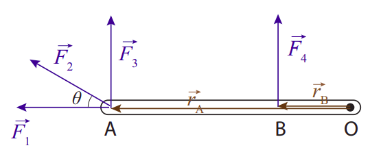
Clearly, the force \(\vec F_1\) will not cause a rotation at all, and accordingly its torque is zero (since it is parallel to \(\vec r_A\)). On the other hand, of all the forces shown, the most effective one is \(\vec F_3\): it is applied the farthest away from O, for the greatest leverage (again, think of your experiences with wrenches). It is also perpendicular to the rod, for maximum effect (\(\sin \theta\) = 1). The force \(\vec F_2\), by contrast, although also applied at the point A is at a disadvantage because of the relatively small angle it makes with \(\vec r_A\). If you imagine breaking it up into components, parallel and perpendicular to the rod, only the perpendicular component (whose magnitude is \(F_2 \sin \theta\)) would be effective at causing a rotation; the other component, the one parallel to the rod, would be wasted, like \(\vec F_1\).

In order to calculate torques, then, we basically need to find, for every force, the component that is perpendicular to the position vector of its point of application. Clearly, for this purpose we can no longer represent an extended body as a mere dot, as we did for the free-body diagrams in Chapter 6. What we need is a more careful sketch of the object, just detailed enough that we can tell how far from the center of rotation and at what angle each force is applied. That kind of diagram is called an extended free-body diagram.

Figure \(\PageIndex{1}\) could be an example of an extended free-body diagram, for an object being acted on by four forces. Typically, though, instead of drawing the vectors \(\vec r_A\) and \(\vec r_B\) we would just indicate their lengths on the diagram (or maybe even leave them out altogether, if we do not want to overload the diagram with detail). I will show a couple of examples of extended free-body diagrams in the next couple of sections.

As indicated above, to calculate the torque of each force acting on an extended object you should use the position vector \(\vec r\) of the point where the force is applied. This is typically unambiguous for contact forces⁴, but what about gravity? In principle, the force of gravity would act on all of the particles making up the body, and we would have to add up all the corresponding torques:

\[ \vec{\tau}^{G}=\vec{r}_{1} \times \vec{F}_{E, 1}^{G}+\vec{r}_{2} \times \vec{F}_{E, 2}^{G}+\ldots \label{eq:9.23} .\]

We can, however, simplify this substantially by noting that (near the surface of the Earth, at any rate), all the forces \(F_{E, 1}^{G}\), \(F_{E, 2}^{G}\) ... point in the same direction (which is to say, down), and they are all proportional to each particle’s mass. If I let the total mass of the object be \(M\), and the total force due to gravity on the object be \(\vec{F}_{E, o b j}^{G}\), then I have \(\vec{F}_{E, 1}^{G}=m_{1} \vec{F}_{E, o b j}^{G} / M\), \(\vec{F}_{E, 2}^{G}=m_{2} \vec{F}_{E, o b j}^{G} / M\),..., and I can rewrite Equation (\ref{eq:9.23}) as

\[ \vec{\tau}^{G}=\frac{m_{1} \vec{r}_{1}+m_{2} \vec{r}_{2}+\ldots}{M} \times \vec{F}_{E, o b j}^{G}=\vec{r}_{c m} \times \vec{F}_{E, o b j}^{G} \label{eq:9.24} \]

where \(\vec r_{cm}\) is the position vector of the object’s center of mass. So to find the torque due to gravity on an extended object, just take the total force of gravity on the object (that is to say, the weight of the object) to be applied at its center of mass. (Obviously, then, the torque of gravity around the center of mass itself will be zero, but in some important cases an object may be pivoted at a point other than its center of mass.)

Coming back to Equation (\ref{eq:9.22}), the main message of this section (other, of course, than the definition of torque itself), is that the rate of change of an object or system’s angular momentum is equal to the net torque due to the external forces. Two special results follow from this one. First, if the net external torque is zero, angular momentum will be conserved, as was the case, in particular, for the collision illustrated earlier, in Figure 9.2.3, between a particle and a rod pivoted at one end. The only external force in that case was the force exerted on the rod, at the pivot point, by the pivot itself, but the torque of that force around that point is obviously zero, since \(\vec r = 0\), so our assumption that the total angular momentum around that point was conserved was legitimate.

Secondly, if \(\vec L = I\vec \omega\) holds, and the moment of inertia \(I\) does not change with time, we can rewrite Equation (\ref{eq:9.22}) as

\[ \vec{\tau}_{\text {ext}, a l l}=I \vec{\alpha} \label{eq:9.25} \]

which is basically the rotational equivalent of Newton’s, second law, \(\vec F = m\vec a\). We will use this extensively in the remainder of this chapter.

Finally, note that situations where the moment of inertia of a system, \(I\), changes with time are relatively easy to arrange for any deformable system. Especially interesting is the case when the external torque is zero, so \(L\) is constant, and a change in \(I\) therefore brings about a change in \(\omega = L/I\): this is how, for instance, an ice-skater can make herself spin faster by bringing her arms closer to the axis of rotation (reducing her \(I\)), and, conversely, slow down her spin by stretching out her arms. This can be done even in the absence of a contact point with the ground: high-board divers, for instance, also spin up in this way when they curl their bodies into a ball. Note that, throughout the dive, the diver’s angular momentum around its center of mass is constant, since the only force acting on him (gravity, neglecting air resistance) has zero torque about that point.

In all the cases just mentioned, the angular momentum is constant, but the rotational kinetic energy changes. This is due to the work done by the internal forces (of the ice-skater’s or the diver’s body), converting some internal energy (such as elastic muscular energy) into rotational kinetic energy, or vice-versa. A convenient expression for a system’s rotational kinetic energy when \(\vec L = I\vec \omega\) holds is

\[ K_{r o t}=\frac{1}{2} I \omega^{2}=\frac{L^{2}}{I} \label{eq:9.26} \]

which shows explicitly how \(K\) would change if \(I\) changed and \(L\) remained constant.

---

³The additional assumption is that the force between any two particles lies along the line connecting the two particles (which means it is parallel or antiparallel to the vector \(\vec{r}_{1}-\vec{r}_{2}\)). In that case, \(\vec{r}_{1} \times \vec{F}_{12}+\vec{r}_{2} \times \vec{F}_{21}=\left(\vec{r}_{1}-\vec{r}_{2}\right) \times \vec{F}_{12}=0\). Most forces in nature satisfy this condition.

⁴Actually, friction forces and normal forces may be “spread out” over a whole surface, but, if the object has enough symmetry, it is usually OK to have them “act” at the midpoint of that surface. This can be proved along the lines of the derivation for gravity that follows.