15.5: Torque on a Magnetic Dipole and Electric Motors

Last updated
Save as PDF

Page ID: 32838

\( \newcommand{\vecs}[1]{\overset { \scriptstyle \rightharpoonup} {\mathbf{#1}} } \) \( \newcommand{\vecd}[1]{\overset{-\!-\!\rightharpoonup}{\vphantom{a}\smash {#1}}} \)\(\newcommand{\id}{\mathrm{id}}\) \( \newcommand{\Span}{\mathrm{span}}\) \( \newcommand{\kernel}{\mathrm{null}\,}\) \( \newcommand{\range}{\mathrm{range}\,}\) \( \newcommand{\RealPart}{\mathrm{Re}}\) \( \newcommand{\ImaginaryPart}{\mathrm{Im}}\) \( \newcommand{\Argument}{\mathrm{Arg}}\) \( \newcommand{\norm}[1]{\| #1 \|}\) \( \newcommand{\inner}[2]{\langle #1, #2 \rangle}\) \( \newcommand{\Span}{\mathrm{span}}\) \(\newcommand{\id}{\mathrm{id}}\) \( \newcommand{\Span}{\mathrm{span}}\) \( \newcommand{\kernel}{\mathrm{null}\,}\) \( \newcommand{\range}{\mathrm{range}\,}\) \( \newcommand{\RealPart}{\mathrm{Re}}\) \( \newcommand{\ImaginaryPart}{\mathrm{Im}}\) \( \newcommand{\Argument}{\mathrm{Arg}}\) \( \newcommand{\norm}[1]{\| #1 \|}\) \( \newcommand{\inner}[2]{\langle #1, #2 \rangle}\) \( \newcommand{\Span}{\mathrm{span}}\)\(\newcommand{\AA}{\unicode[.8,0]{x212B}}\)

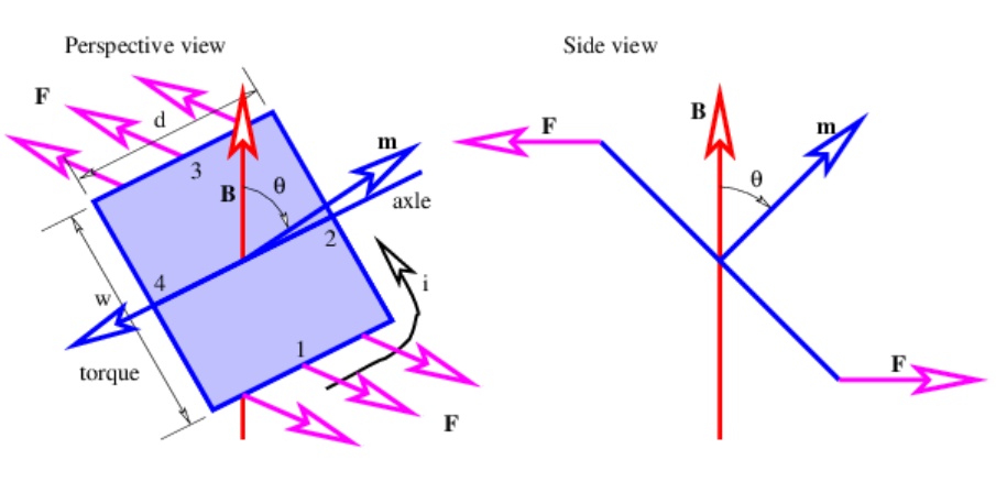
Figure 15.6 shows a rectangular loop of wire mounted on an axle in a magnetic field. A current i exists in the loop as shown. The currents in loop segments 2 and 4 experience a force parallel to the axle. These forces generate no net torque. However, the magnetic forces on loop segments 1 and 3 are each \(F=\text { id } B\) in magnitude, where \(B=|\mathbf{B}|\) is the magnitude of the magnetic field.

Figure 15.6: Perspective and side views of a rectangular loop of wire mounted on an axle in a magnetic field. Forces on the currents in loop segments 1 and 3 generate a torque about the axle.

Together these forces generate a counterclockwise torque about the axle equal to \(\mathrm{T}=2 \mathrm{~F}(\mathrm{w} / 2) \sin (\theta)=\operatorname{iwd} \mathrm{B} \sin (\theta)\). This can be represented in vector form as

\[\boldsymbol{\tau}=\mathbf{m} \times \mathbf{B}\label{15.15}\]

where \(\mathbf{m}\) is a vector with magnitude \(iwd\) and direction normal to the loop as shown in figure 15.6. The vector \(\mathbf{m}\) is called the magnetic dipole moment.

The loop can actually be any shape, not just rectangular. In the general case the magnitude of the magnetic moment equals the current i times the area \(S\) of the loop:

\[|\mathbf{m}|=i S \quad \text { (magnetic dipole moment). }\label{15.16}\]

In the above example the area is \(\mathrm{S}=\text { wd. }\). The direction of m is determined by the right hand rule; curl the fingers on your right hand around the loop in the direction of the current and your thumb points in the direction of \(m\).

In analogy with the electric dipole in an electric field, the potential energy of a magnetic dipole in a magnetic field is

\[U=-\mathbf{m} \cdot \mathbf{B}\label{15.17}\]

Figure 15.6 illustrates the principle of an electric motor. A motor consists of multiple loops of wire on an axle carrying a current in a magnetic field. The torque on the axle turns the loops so that the magnetic moment is parallel to the field. The angular momentum of the loops carries the rotation of the axle through the zero torque region, which occurs when the magnetic moment is either perfectly parallel or perfectly anti-parallel (i. e., pointing in the opposite direction) to the field. At this point either the magnetic field is reversed by some mechanism or the magnetic dipole is reversed by making the current circulate around the loops in the opposite direction. The torque due to the magnetic force then turns the axle through another half-turn, whereupon the field or the magnetic moment is again reversed, and so on.