15.6: Electric Generators and Faraday’s Law

As was shown earlier, the electric field is derived from two different sources, spatial derivatives of the scalar potential and time derivatives of the vector potential:

\[E_{x}=-\frac{\partial \phi}{\partial x}-\frac{\partial A_{x}}{\partial t}, \quad E_{y}=-\frac{\partial \phi}{\partial y}-\frac{\partial A_{y}}{\partial t}, \quad E_{z}=-\frac{\partial \phi}{\partial z}-\frac{\partial A_{z}}{\partial t}\label{15.18}\]

In time independent situations the vector potential part drops out and we are left with a dependence only on the scalar potential. In this case a particle with charge \(q\) has an electrostatic potential energy \(\mathrm{U}=\mathrm{q} \phi \text { , }\), which means that the electric force is conservative. However, in the time dependent situation there is no guarantee that the part of the electric field derived from the vector potential will be conservative.

Figure 15.7: Illustration of the electric field pattern \(E\) = (-\(Cy,Cx, \) 0) (small arrows). A charged particle moving in a circle as shown continually gains energy.

An example of a non-conservative electric field occurs when we have

\[\mathbf{A}=(C y t,-C x t, 0), \quad \phi=0\label{15.19}\]

where \(C\) is a constant. In this case the electric and magnetic fields are

\[\mathbf{E}=(-C y, C x, 0), \quad \mathbf{B}=(0,0,-2 C t)\label{15.20}\]

The magnetic field points in the -\(z\) direction and increases in magnitude with time. The electric field vectors are shown in figure 15.7. Notice that a positively charged particle moving in a counterclockwise circle as shown is continually being accelerated in the direction of motion, and is therefore continually gaining energy. This is impossible with a conservative force.

How much energy is gained by a particle with charge \(q\) moving in a complete circle of radius \(R\) under the above circumstances? The magnitude of the electric field at this radius is \(\mathrm{E}=\mathrm{CR}\), so the force on the particle is \(\mathrm{F}=\mathrm{gCR}\). The circumference of the circle is \(2 \pi R\), so the total work done by the electric field in one revolution is just \(\Delta \mathrm{W}=2 \pi \mathrm{RF}=2 \pi \mathrm{CR}^{2}=2 \mathrm{gCS}, \text { where } \mathrm{S}=\mathrm{nR}^{2}\) is the area of the circle. Let us define \(\Delta \mathrm{V}=\Delta \mathrm{W} / \mathrm{q}=2 \mathrm{CS}\). For historical reasons this is called the electromotive force or EMF. This is deceptive terminology, because in fact \(\Delta \mathrm{V}\) doesn’t have the dimensions of force — it is really just the work per unit charge done on a particle making a single loop around the circle in figure 15.7.

Recall that the \(z\) component of the magnetic field in this case is \(\mathrm{B}_{\mathrm{z}}=-2 \mathrm{Ct}\). Note that the time derivative of the magnetic field is just \(\partial \mathrm{B}_{\mathrm{z}} / \partial \mathrm{t}=-2 \mathrm{C}\). Comparison with the equation for electromotive force shows us that

\[\Delta V=-\frac{\partial B_{z}}{\partial t} S=-\frac{\partial B_{z} S}{\partial t}\label{15.21}\]

where the area is brought inside the time derivative since it is constant in time.

Figure 15.8: Sketch illustrating Faraday’s law for a fixed loop. The arrows passing through the loop indicate the direction of the time rate of change of the magnetic field. The arrow going around the loop indicates the direction a positive charge would be pushed by the electric field.

Notice that the argument of the time derivative in the above equation is the component of \(B\) perpendicular to the plane of the loop. The loop area multiplied by the normal component of \(B\) is the magnetic flux through the loop: \(\Phi_{\mathrm{B}} \equiv \mathrm{B}_{\text {normal }} \mathrm{S}\). The generalization of equation (\ref{15.21}) for any loop fixed in space is expressed as

\[\Delta V=-\left(\frac{d \Phi_{B}}{d t}\right)_{\text {fixed }} \quad(\text { fixed loop })\label{15.22}\]

It is valid for arbitrary loop and magnetic field configurations, not just for the simple case we have been investigating.

The minus sign in equation (\ref{15.22}) means the following: If the fingers on your right hand curl around the loop in the direction opposite to the direction that causes a positive charge to gain energy, then your thumb points in the direction of the time rate of change of the magnetic flux passing through the loop. This is illustrated in figure 15.8.

If a loop is changing size or shape with time, then the magnetic force also acts on charges in the loop. The work per unit charge done in a segment \(j \)of the loop defined by the displacement vector \(\Delta \mathbf{I}_{j}\) is

\[\Delta V_{j}=\left(\mathbf{v}_{j} \times \mathbf{B}_{j}\right) \cdot \Delta \mathbf{l}_{j}\label{15.23}\]

where \(\mathbf{v}_{j}\) is the velocity with which the loop segment is moving and \(\mathbf{B}_{j}\) is the magnetic field at the location of the segment. To get the total EMF around the loop due to the magnetic force, the \(\Delta V_{j}\) values from each segment must simply be summed up and added to the right side of equation (\ref{15.22}):

\[\Delta V=-\left(\frac{d \Phi_{B}}{d t}\right)_{\text {fixed }}+\sum_{i}\left(\mathbf{v}_{j} \times \mathbf{B}_{j}\right) \cdot \Delta \mathbf{l}_{j}\label{15.24}\]

It turns out that the part of ΔV resulting from a moving or deforming loop equals minus the time rate of change of magnetic flux through the loop due solely to loop movement and deformation. Therefore, we can rewrite equation (\ref{15.24}) in the more compact form

\[\Delta V=-\frac{d \Phi_{B}}{d t} \quad \text { Faraday's law. }\label{15.25}\]

where the time derivative of the magnetic flux now includes both changes in the magnetic field and changes in the position, shape, and orientation of the loop. This is called Faraday’s law, even though it is a hybrid of equation (\ref{15.22}), which is Faraday’s law as generally defined in advanced physics and the Lorentz force law as expressed in equation (\ref{15.23}).

Figure 15.9: Rotating wire loop in a magnetic field. At the instant illustrated the magnetic flux is increasing with time, which means that an EMF tends to drive a current as illustrated.

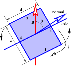
The electric generator is perhaps the best known application of Faraday’s law. Figure 15.9 shows a rectangular loop of wire fixed to an axle that rotates at an angular rate Ω. The magnetic flux through the loop thus varies with time according to \(\Phi_{\mathrm{B}}=\mathrm{wdB} \cos (\theta)=\mathrm{wdB} \cos (\Omega \mathrm{t})\). The EMF around the loop is thus

\[\Delta V=-\frac{d \Phi_{B}}{d t}=\Omega w d B \sin (\Omega t)\label{15.26}\]

In a real generator there are many loops forming a coil of wire and the ends of the coil are brought out through the axle so that the resulting current can be tapped for practical use.