
16.5: Moving Charge and Magnetic Fields


- Last updated
- Nov 6, 2024
- Save as PDF

( \newcommand{\kernel}{\mathrm{null}\,}\)
We have shown that electric charge generates both electric and magnetic fields, but the latter result only from moving charge. If we have the scalar potential due to a static configuration of charge, we can use this result to find the magnetic field if this charge is set in motion. Since the four-potential is tangent to the particle’s world line, and hence is parallel to the time axis in the reference frame in which the charged particle is stationary, we know how to resolve the space and time components of the four-potential in the reference frame in which the charge is moving.
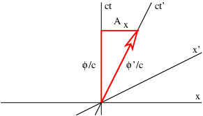
Figure 16.4 illustrates this process. For a particle moving in the +x direction at speed v, the slope of the time axis in the primed frame is just c/v . The four-potential vector has this same slope, which means that the space and time components of the four-potential must now appear as shown in Figure 16.5.4:. If the scalar potential in the primed frame is ϕ′, then in the unprimed frame it is ϕ, and the x component of the vector potential is AX. Using the space time Pythagorean theorem, ϕ′2/c2=ϕ2/c2−A2x2, and relating slope of the ct′ axis to the components of the four-potential, c/v=(ϕ/c)/Ax, it is possible to show that
ϕ=γϕ′Ax=vγϕ′/c2
where
γ=1(1−v2/c2)1/2
Thus, the principles of special relativity allow us to obtain the full four-potential for a moving configuration of charge if the scalar potential is known for the charge when it is stationary. From this we can derive the electric and magnetic fields for the moving charge.
Moving Line of Charge
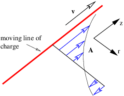
As an example of this procedure, let us see if we can determine the magnetic field from a line of charge with linear charge density in its own rest frame of λ′, aligned along the z axis. The line of charge is moving in a direction parallel to itself. From equation (???) we see that the scalar potential a distance r from the z axis is
ϕ′=−λ′2πϵ0ln(r)
in a reference frame moving with the charge. The z component of the vector potential in the stationary frame is therefore
Az=−λ′vγ2πϵ0c2ln(r)
by equation (???), with all other components being zero. This is illustrated in figure 16.5.
We infer that
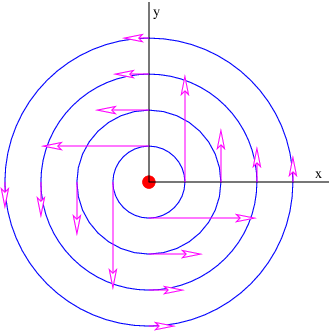
Bx=∂Az∂y=−λ′vγy2πϵ0c2r2By=−∂Az∂x=λ′vγx2πϵ0c2r2Bz=0
where we have used r2=x2+y2. The resulting field is illustrated in Figure 16.5.6:. The field lines circle around the line of moving charge and the magnitude of the magnetic field is
B=(B2x+B2y)1/2=λ′vγ2πϵ0c2r
There is an interesting relativistic effect on the charge density λ′, which is defined in the co-moving or primed reference frame. In the unprimed frame the charges are moving at speed v and therefore undergo a Lorentz contraction in the z direction. This decreases the charge spacing by a factor of γ and therefore increases the charge density as perceived in the unprimed frame to a value λ=γλ′.
We also define a new constant μ0≡1/(ϵ0c2). This is called the permeability of free space. This constant has the assigned value μ0=4π×10−7 N s2C−2. The value of ϵ0=1/(μ0c2) is actually derived from this assigned value and the measured value of the speed of light. The reasons for this particular way of dealing with the constants of electromagnetism are obscure, but have to do with making it easy to relate the values of constants to the experiments used in determining them.
With the above substitutions, the magnetic field equation becomes
B=μ0λv2πr
The combination λv is called the current and is symbolized by i. The current is the charge per unit time passing a point and is a fundamental quantity in electric circuits. The magnetic field written in terms of the current flowing along the z axis is
B=μ0i2πr (straight wire).
Moving Sheet of Charge
As another example we consider a uniform infinite sheet of charge in the x - y plane with charge density σ ′. The charge is moving in the +x direction with speed v. As we showed in the section on Gauss’s law for electricity, the electric field for this sheet of charge in the co-moving reference frame is in the z direction and has the value
E′z=σ′2ϵ0sgn(z)
where we define
sgn(z)≡{−1z<00z=01z>0
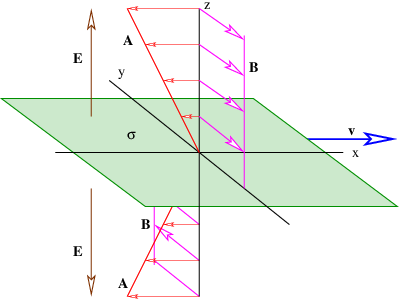
The sgn(z) function is used to indicate that the electric field points upward above the sheet of charge and downward below it (see Figure 16.5.7:).
The scalar potential in this frame is
ϕ′=−σ′|z|2ϵ0
In the stationary reference frame in which the sheet of charge is moving in the x direction, the scalar potential and the x component of the vector potential are
ϕ=−γσ′|z|2ϵ0=−σ|z|2ϵ0Ax=−vγσ′|z|2ϵ0c2=−vσ|z|2ϵ0c2
according to Equation ???, where σ=γσ′ is the charge density in the stationary frame. The other components of the vector potential are zero. We calculate the magnetic field as
Bx=0By=dAxdz=−vσ2ϵ0c2sgn(z)Bz=0
where sgn(z) is defined as before. The vector potential and the magnetic field are shown in Figure 16.5.7:. Note that the magnetic field points normal to the direction of motion of the charge but parallel to the sheet. It points in opposite directions on opposite sides of the sheet of charge.