16.6: Electromagnetic Radiation

We have found so far that stationary charge produces an electric field while moving charge produces a magnetic field. It turns out that accelerated charge produces electromagnetic radiation. Electromagnetic radiation is nothing more than one or more photons that have zero mass, and are therefore real, not virtual.

Figure 16.8: Feynman diagrams for two common processes that produce real photons and hence electromagnetic radiation. The process in the left panel is possible only if the mass of particle A is greater than the mass of particle B, due to the conservation of energy. Solid lines represent electrons while dashed lines represent photons. Particles are taken to be real unless otherwise labeled.

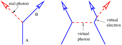
Acceleration of a charged particle is needed to produce radiation because of the conservation of energy and momentum. The left panel of figure 16.8 shows why. Since a photon carries off energy and momentum, conservation means that the energy and momentum of the emitting particle change due to the emission of a photon. This corresponds in classical mechanics to an acceleration.

The process in the left panel of figure 16.8 actually cannot occur if particles A and B have the same mass. If the mass of the outgoing particle B is less than the mass of the incoming particle A, then this reaction can and does occur. An example is the decay of an atom from a higher energy state to a lower energy state (and hence lower mass), accompanied by the emission of a photon.

Another type of reaction that can generate radiation occurs when two charged particles (say, electrons) collide, as illustrated in the right panel of figure 16.8. In an elastic collision both electrons are real both before and after the photon transfer. However, it is possible for one of the electrons to have a virtual mass that is greater than the normal electron mass after the collision, which means that it is free to decay to a real electron plus a real photon.

We now try to understand the characteristics of free electromagnetic radiation. In our studies of waves we found it easiest to examine plane waves. We will follow this path here, writing the four-potential for an electromagnetic plane wave moving in the \(x \) direction as

\[\underline{a}=(\mathbf{A}, \phi / c)=\left(\mathbf{A}_{0}, \phi_{0} / c\right) \cos \left(k_{x} x-\omega t\right),\label{16.26}\]

where \(a\) ₀ = (\(A\) ₀\(,ϕ\) ₀\(∕c\) ) is a constant four-vector representing the direction and maximum amplitude of the four-potential, and \(k\) _x and \(\omega\) are the wavenumber and the angular frequency of the wave. Since the real photon is massless, we have \(\omega=k_{x} c\) in this case. Virtual photons are not subject to this constraint.

By substituting \(A\) and \(\phi\) from Equation \ref{16.26} into the Lorenz condition, we find that

\[k_{x} A_{x}-\omega \phi / c^{2}=0 \quad \text { (Lorenz condition for plane wave). } \label{16.27}\]

Thus, the Lorenz condition requires that the scalar potential \(\phi\) be related to the \(x\) or longitudinal component of the vector potential, \(A\)_x, i. e., the component pointing in the direction of wave propagation. The transverse components , \(A\)_y and \(A\)_z, are unconstrained by the Lorenz condition, since they don’t depend on \(y \) and \(z\).

Using equations for the electric and magnetic field, as well as equations (\ref{16.26}) and (\ref{16.27}), we can now find \(E\) and \(B\) in an electromagnetic plane wave:

\[B = (0,kxA0z,- kxA0y )sin(kxx - ωt) \label{16.28}\]

\[E = (kxϕ0 - ωA0x, - ωA0y,- ωA0z )sin(kxx - ωt ). \label{16.29}\]

The electric field has a longitudinal or \(x\) component proportional to \(\mathrm{k}_{\mathrm{x}} \phi_{0}-\omega \mathrm{A}_{0 \mathrm{x}}=-\omega\left(\phi_{0} / \mathrm{c}-\mathrm{A}_{0 \mathrm{x}}\right)\). However, comparison with equation (\ref{16.27}) shows that \(E_{x}=0\) as long as \(\omega / \mathrm{k}_{\mathrm{x}}=\mathrm{c}_{\boldsymbol{}}\), i. e., as long as the photons travel at the speed of light, \(c\). Thus, virtual photons, i. e., those that have a non-zero mass and therefore travel at a speed other than that of light, can have a non-zero longitudinal component of the electric field, but real photons cannot.

The dot product of the electric and magnetic fields in a plane wave is \(\mathbf{E} \cdot \mathbf{B}=0,\), as can be verified from equations (\ref{16.28}) and (\ref{16.29}). This means that \(E\) and \(B\) are perpendicular to each other. Furthermore, both E and B are perpendicular to the direction of wave motion for real photons.

Figure 16.9: Electric and magnetic fields in a horizontally polarized plane wave, i. e., with \(A\) _z = 0, moving in the direction of the large arrow. The left panel shows how the electric and magnetic fields point, while the right panel shows the distribution of the magnetic field in space.

Figure 16.9 shows the electric and magnetic fields for real photons in the special case where \(A\) _z = 0. The electric field points in the same direction as the transverse part of the vector potential, while the magnetic field points in the other transverse direction. The ratio of the magnitudes of the electric and magnetic fields is easily inferred from equations (\ref{16.28}) and (\ref{16.29}):

\[\frac{|\mathbf{E}|}{|\mathbf{B}|}=\frac{\omega\left(A_{y}^{2}+A_{z}^{2}\right)^{1 / 2} \sin \left(k_{x} x-\omega t\right)}{k_{x}\left(A_{z}^{2}+A_{y}^{2}\right)^{1 / 2} \sin \left(k_{x} x-\omega t\right)}=\frac{\omega}{k_{x}}=c \label{16.30}\]

Notice that the electric and magnetic fields for a wave do not depend on the longitudinal component of the vector potential, \(A\)_x. This is because the Lorenz condition forces \(A\)_x to cancel with the term containing \(\phi\) in the expression for \(E\)_x.