5.3: Principle of Relativity Applied

Returning to the phase of a wave, we immediately see that

\[\phi=\mathbf{k} \cdot \mathbf{x}-\omega t=\mathbf{k} \cdot \mathbf{x}-(\omega / c)(c t)=\underline{k} \cdot \underline{x} .\label{5.7}\]

Thus, a compact way to rewrite equation (5.2.2) is

\[A(\underline{x})=A_{0} \sin (\underline{k} \cdot \underline{x})\label{5.8}\]

Since x is known to be a four-vector and since the phase of a wave is known to be a scalar independent of reference frame, it follows that k is also a four-vector rather than just a set of numbers. Thus, the square of the length of the wave four-vector must also be a scalar independent of reference frame:

\[\underline{k} \cdot \underline{k}=\mathbf{k} \cdot \mathbf{k}-\omega^{2} / c^{2}=\text { const. }\label{5.9}\]

Figure 5.2: Resolution of a four-vector into components in two different reference frames.

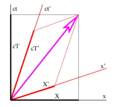
Let us review precisely what this means. As figure 5.2 shows, we can resolve a position four-vector into components in two different reference frames, \(\underline{x}=(X, c T)=\left(X^{\prime}, c T^{\prime}\right)\). However, even though \(X \neq X^{\prime} \text { and } T \neq T^{\prime}\), the vector lengths computed from these two sets of components are necessarily the same: \(\underline{x} \cdot \underline{x}=X^{2}-c^{2} T^{2}=X^{\prime 2}-c^{2} T^{\prime 2}\).

Applying this to the wave four-vector, we infer that

\[k^{2}-\omega^{2} / c^{2}=k^{2}-\omega^{\prime 2} / c^{2}=\text { const. }\label{5.10}\]

where the unprimed and primed values of k and ω refer to the components of the wave four-vector in two different reference frames.

Up to now, this argument applies to any wave. However, waves can be divided into two categories, those for which a “special” reference frame exists, and those for which there is no such special frame. As an example of the former, sound waves look simplest in the reference frame in which the gas carrying the sound is stationary. The same is true of light propagating through a material medium with an index of refraction not equal to unity. In both cases the speed of the wave is the same in all directions only in the frame in which the material medium is stationary.

Suppose we have a machine that produces a wave with wavenumber k and frequency ω in its own rest frame. If we observe the wave from a moving reference frame, the wavenumber and frequency will be different, say, \(\mathrm{k}^{\prime}\) and \(\omega^{\prime}\). However, these quantities will be related by equation (\ref{5.10}).

Up to this point the argument applies to any wave whether a special reference frame exists or not; the observed changes in wavenumber and frequency have nothing to do with the wave itself, but are just consequences of how we have chosen to observe it. However, if there is no special reference frame for the type of wave under consideration, then the same result can be obtained by keeping the observer stationary and moving the wave-producing machine in the opposite direction. By moving it at various speeds, any desired value of \(\mathrm{k}^{\prime}\) can be obtained in the initial reference frame (as opposed to some other frame), and the resulting value of \(\omega^{\prime}\) can be computed using equation (\ref{5.10}).

This is actually an amazing result. We have shown on the basis of the principle of relativity that any wave type for which no special reference frame exists can be made to take on a full range of frequencies and wavenumbers in any given reference frame, and furthermore that these frequencies and wavenumbers obey

\[\omega^{2}=k^{2} c^{2}+\mu^{2}\label{5.11}\]

Equation (\ref{5.11}) comes from solving equation (5.10) for \(\omega^{2}\) and the constant \(\mu^{2}\) equals the constant in equation (\ref{5.10}) times -c². Equation (\ref{5.11}) relates frequency to wavenumber and therefore is the dispersion relation for such waves. We call waves which have no special reference frame and therefore necessarily obey equation (\ref{5.11}) relativistic waves. The only difference in the dispersion relations between different types of relativistic waves is the value of the constant μ. The meaning of this constant will become clear later.