14.7: Fluid Dynamics
- Page ID
- 4059
\( \newcommand{\vecs}[1]{\overset { \scriptstyle \rightharpoonup} {\mathbf{#1}} } \)
\( \newcommand{\vecd}[1]{\overset{-\!-\!\rightharpoonup}{\vphantom{a}\smash {#1}}} \)
\( \newcommand{\dsum}{\displaystyle\sum\limits} \)
\( \newcommand{\dint}{\displaystyle\int\limits} \)
\( \newcommand{\dlim}{\displaystyle\lim\limits} \)
\( \newcommand{\id}{\mathrm{id}}\) \( \newcommand{\Span}{\mathrm{span}}\)
( \newcommand{\kernel}{\mathrm{null}\,}\) \( \newcommand{\range}{\mathrm{range}\,}\)
\( \newcommand{\RealPart}{\mathrm{Re}}\) \( \newcommand{\ImaginaryPart}{\mathrm{Im}}\)
\( \newcommand{\Argument}{\mathrm{Arg}}\) \( \newcommand{\norm}[1]{\| #1 \|}\)
\( \newcommand{\inner}[2]{\langle #1, #2 \rangle}\)
\( \newcommand{\Span}{\mathrm{span}}\)
\( \newcommand{\id}{\mathrm{id}}\)
\( \newcommand{\Span}{\mathrm{span}}\)
\( \newcommand{\kernel}{\mathrm{null}\,}\)
\( \newcommand{\range}{\mathrm{range}\,}\)
\( \newcommand{\RealPart}{\mathrm{Re}}\)
\( \newcommand{\ImaginaryPart}{\mathrm{Im}}\)
\( \newcommand{\Argument}{\mathrm{Arg}}\)
\( \newcommand{\norm}[1]{\| #1 \|}\)
\( \newcommand{\inner}[2]{\langle #1, #2 \rangle}\)
\( \newcommand{\Span}{\mathrm{span}}\) \( \newcommand{\AA}{\unicode[.8,0]{x212B}}\)
\( \newcommand{\vectorA}[1]{\vec{#1}} % arrow\)
\( \newcommand{\vectorAt}[1]{\vec{\text{#1}}} % arrow\)
\( \newcommand{\vectorB}[1]{\overset { \scriptstyle \rightharpoonup} {\mathbf{#1}} } \)
\( \newcommand{\vectorC}[1]{\textbf{#1}} \)
\( \newcommand{\vectorD}[1]{\overrightarrow{#1}} \)
\( \newcommand{\vectorDt}[1]{\overrightarrow{\text{#1}}} \)
\( \newcommand{\vectE}[1]{\overset{-\!-\!\rightharpoonup}{\vphantom{a}\smash{\mathbf {#1}}}} \)
\( \newcommand{\vecs}[1]{\overset { \scriptstyle \rightharpoonup} {\mathbf{#1}} } \)
\( \newcommand{\vecd}[1]{\overset{-\!-\!\rightharpoonup}{\vphantom{a}\smash {#1}}} \)
\(\newcommand{\avec}{\mathbf a}\) \(\newcommand{\bvec}{\mathbf b}\) \(\newcommand{\cvec}{\mathbf c}\) \(\newcommand{\dvec}{\mathbf d}\) \(\newcommand{\dtil}{\widetilde{\mathbf d}}\) \(\newcommand{\evec}{\mathbf e}\) \(\newcommand{\fvec}{\mathbf f}\) \(\newcommand{\nvec}{\mathbf n}\) \(\newcommand{\pvec}{\mathbf p}\) \(\newcommand{\qvec}{\mathbf q}\) \(\newcommand{\svec}{\mathbf s}\) \(\newcommand{\tvec}{\mathbf t}\) \(\newcommand{\uvec}{\mathbf u}\) \(\newcommand{\vvec}{\mathbf v}\) \(\newcommand{\wvec}{\mathbf w}\) \(\newcommand{\xvec}{\mathbf x}\) \(\newcommand{\yvec}{\mathbf y}\) \(\newcommand{\zvec}{\mathbf z}\) \(\newcommand{\rvec}{\mathbf r}\) \(\newcommand{\mvec}{\mathbf m}\) \(\newcommand{\zerovec}{\mathbf 0}\) \(\newcommand{\onevec}{\mathbf 1}\) \(\newcommand{\real}{\mathbb R}\) \(\newcommand{\twovec}[2]{\left[\begin{array}{r}#1 \\ #2 \end{array}\right]}\) \(\newcommand{\ctwovec}[2]{\left[\begin{array}{c}#1 \\ #2 \end{array}\right]}\) \(\newcommand{\threevec}[3]{\left[\begin{array}{r}#1 \\ #2 \\ #3 \end{array}\right]}\) \(\newcommand{\cthreevec}[3]{\left[\begin{array}{c}#1 \\ #2 \\ #3 \end{array}\right]}\) \(\newcommand{\fourvec}[4]{\left[\begin{array}{r}#1 \\ #2 \\ #3 \\ #4 \end{array}\right]}\) \(\newcommand{\cfourvec}[4]{\left[\begin{array}{c}#1 \\ #2 \\ #3 \\ #4 \end{array}\right]}\) \(\newcommand{\fivevec}[5]{\left[\begin{array}{r}#1 \\ #2 \\ #3 \\ #4 \\ #5 \\ \end{array}\right]}\) \(\newcommand{\cfivevec}[5]{\left[\begin{array}{c}#1 \\ #2 \\ #3 \\ #4 \\ #5 \\ \end{array}\right]}\) \(\newcommand{\mattwo}[4]{\left[\begin{array}{rr}#1 \amp #2 \\ #3 \amp #4 \\ \end{array}\right]}\) \(\newcommand{\laspan}[1]{\text{Span}\{#1\}}\) \(\newcommand{\bcal}{\cal B}\) \(\newcommand{\ccal}{\cal C}\) \(\newcommand{\scal}{\cal S}\) \(\newcommand{\wcal}{\cal W}\) \(\newcommand{\ecal}{\cal E}\) \(\newcommand{\coords}[2]{\left\{#1\right\}_{#2}}\) \(\newcommand{\gray}[1]{\color{gray}{#1}}\) \(\newcommand{\lgray}[1]{\color{lightgray}{#1}}\) \(\newcommand{\rank}{\operatorname{rank}}\) \(\newcommand{\row}{\text{Row}}\) \(\newcommand{\col}{\text{Col}}\) \(\renewcommand{\row}{\text{Row}}\) \(\newcommand{\nul}{\text{Nul}}\) \(\newcommand{\var}{\text{Var}}\) \(\newcommand{\corr}{\text{corr}}\) \(\newcommand{\len}[1]{\left|#1\right|}\) \(\newcommand{\bbar}{\overline{\bvec}}\) \(\newcommand{\bhat}{\widehat{\bvec}}\) \(\newcommand{\bperp}{\bvec^\perp}\) \(\newcommand{\xhat}{\widehat{\xvec}}\) \(\newcommand{\vhat}{\widehat{\vvec}}\) \(\newcommand{\uhat}{\widehat{\uvec}}\) \(\newcommand{\what}{\widehat{\wvec}}\) \(\newcommand{\Sighat}{\widehat{\Sigma}}\) \(\newcommand{\lt}{<}\) \(\newcommand{\gt}{>}\) \(\newcommand{\amp}{&}\) \(\definecolor{fillinmathshade}{gray}{0.9}\)- Describe the characteristics of flow
- Calculate flow rate
- Describe the relationship between flow rate and velocity
- Explain the consequences of the equation of continuity to the conservation of mass
The first part of this chapter dealt with fluid statics, the study of fluids at rest. The rest of this chapter deals with fluid dynamics, the study of fluids in motion. Even the most basic forms of fluid motion can be quite complex. For this reason, we limit our investigation to ideal fluids in many of the examples. An ideal fluid is a fluid with negligible viscosity. Viscosity is a measure of the internal friction in a fluid; we examine it in more detail in Viscosity and Turbulence. In a few examples, we examine an incompressible fluid—one for which an extremely large force is required to change the volume—since the density in an incompressible fluid is constant throughout.
Characteristics of Flow
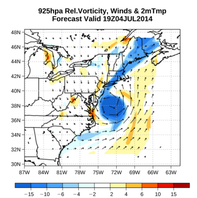
Velocity vectors are often used to illustrate fluid motion in applications like meteorology. For example, wind—the fluid motion of air in the atmosphere—can be represented by vectors indicating the speed and direction of the wind at any given point on a map. Figure \(\PageIndex{1}\) shows velocity vectors describing the winds during Hurricane Arthur in 2014.

Another method for representing fluid motion is a streamline. A streamline represents the path of a small volume of fluid as it flows. The velocity is always tangential to the streamline. The diagrams in Figure \(\PageIndex{2}\) use streamlines to illustrate two examples of fluids moving through a pipe. The first fluid exhibits a laminar flow (sometimes described as a steady flow), represented by smooth, parallel streamlines. Note that in the example shown in part (a), the velocity of the fluid is greatest in the center and decreases near the walls of the pipe due to the viscosity of the fluid and friction between the pipe walls and the fluid. This is a special case of laminar flow, where the friction between the pipe and the fluid is high, known as no slip boundary conditions. The second diagram represents turbulent flow, in which streamlines are irregular and change over time. In turbulent flow, the paths of the fluid flow are irregular as different parts of the fluid mix together or form small circular regions that resemble whirlpools. This can occur when the speed of the fluid reaches a certain critical speed.

Flow Rate and its Relation to Velocity
The volume of fluid passing by a given location through an area during a period of time is called flow rate \(Q\), or more precisely, volume flow rate. In symbols, this is written as
\[Q = \frac{dV}{dt} \label{14.13}\]
where \(V\) is the volume and \(t\) is the elapsed time. In Figure \(\PageIndex{3}\), the volume of the cylinder is \(Ax\), so the flow rate is
\[Q = \frac{dV}{dt} = \frac{d}{dt} (Ax) = A \frac{dx}{dt} = Av \ldotp\]
The SI unit for flow rate is m3/s, but several other units for \(Q\) are in common use, such as liters per minute (L/min). Note that a liter (L) is 1/1000 of a cubic meter or 1000 cubic centimeters (10−3 m3 or 103 cm3).

Flow rate and velocity are related, but quite different, physical quantities. To make the distinction clear, consider the flow rate of a river. The greater the velocity of the water, the greater the flow rate of the river. But flow rate also depends on the size and shape of the river. A rapid mountain stream carries far less water than the Amazon River in Brazil, for example. Figure \(\PageIndex{3}\) illustrates the volume flow rate. The volume flow rate is \(Q = \frac{dV}{dt} = Av\), where A is the cross-sectional area of the pipe and v is the magnitude of the velocity.
The precise relationship between flow rate \(Q\) and average speed \(v\) is
\[Q = Av,\]
where \(A\) is the cross-sectional area and \(v\) is the average speed. The relationship tells us that flow rate is directly proportional to both the average speed of the fluid and the cross-sectional area of a river, pipe, or other conduit. The larger the conduit, the greater its cross-sectional area. Figure \(\PageIndex{3}\) illustrates how this relationship is obtained. The shaded cylinder has a volume \(V = Ad\), which flows past the point \(P\) in a time \(t\). Dividing both sides of this relationship by \(t\) gives
\[\frac{V}{t} = \frac{Ad}{t} \ldotp \label{eq14.14A} \]
We note that \(Q = \frac{V}{t}\) and the average speed is \(v = \frac{d}{t}\). Thus Equation \ref{eq14.14A} becomes
\[Q = Av.\]
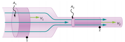
Figure \(\PageIndex{4}\) shows an incompressible fluid flowing along a pipe of decreasing radius. Because the fluid is incompressible, the same amount of fluid must flow past any point in the tube in a given time to ensure continuity of flow. The flow is continuous because they are no sources or sinks that add or remove mass, so the mass flowing into the pipe must be equal the mass flowing out of the pipe. In this case, because the cross-sectional area of the pipe decreases, the velocity must necessarily increase. This logic can be extended to say that the flow rate must be the same at all points along the pipe. In particular, for arbitrary points 1 and 2,
\[\begin{split} Q_{1} & = Q_{2}, \\ A_{1} v_{1} & = A_{2} v_{2} \ldotp \end{split} \label{14.14}\]
This is called the equation of continuity and is valid for any incompressible fluid (with constant density). The consequences of the equation of continuity can be observed when water flows from a hose into a narrow spray nozzle: It emerges with a large speed—that is the purpose of the nozzle. Conversely, when a river empties into one end of a reservoir, the water slows considerably, perhaps picking up speed again when it leaves the other end of the reservoir. In other words, speed increases when cross-sectional area decreases, and speed decreases when cross-sectional area increases.

Since liquids are essentially incompressible, the equation of continuity is valid for all liquids. However, gases are compressible, so the equation must be applied with caution to gases if they are subjected to compression or expansion.
A nozzle with a diameter of 0.500 cm is attached to a garden hose with a radius of 0.900 cm. The flow rate through hose and nozzle is 0.500 L/s. Calculate the speed of the water:
- in the hose and
- in the nozzle.
Strategy
We can use the relationship between flow rate and speed to find both speeds. We use the subscript 1 for the hose and 2 for the nozzle.
Solution
- We solve the flow rate equation for speed and use \(\pi r_{1}^{2}\) for the cross-sectional area of the hose, obtaining $$v = \frac{Q}{A} = \frac{Q}{\pi r_{1}^{2}} \ldotp$$ Substituting values and using appropriate unit conversions yields $$v = \frac{(0.500\; L/s)(10^{-3}\; m^{3}/L)}{(3.14)(9.00 \times 10^{-3}\; m)^{2}} = 1.96\; m/s \ldotp$$
- We could repeat this calculation to find the speed in the nozzle v2, but we use the equation of continuity to give a somewhat different insight. The equation states $$A_{1} v_{1} = A_{2} v_{2} \ldotp$$Solving for v2 and substituting \(\pi r^{2}\) for the cross-sectional area yields $$v_{2} = \frac{A_{1}}{A_{2}} v_{1} = \frac{\pi r_{1}^{2}}{\pi r_{2}^{2}} v_{1} = \frac{r_{1}^{2}}{r_{2}^{2}} v_{1} \ldotp$$ Substituting known values, $$v_{2} = \frac{(0.900\; cm)^{2}}{(0.250\; cm)^{2}} (1.96\; m/s) = 25.5\; m/s \ldotp$$
Significance
A speed of 1.96 m/s is about right for water emerging from a hose with no nozzle. The nozzle produces a considerably faster stream merely by constricting the flow to a narrower tube.
The solution to the last part of the example shows that speed is inversely proportional to the square of the radius of the tube, making for large effects when radius varies. We can blow out a candle at quite a distance, for example, by pursing our lips, whereas blowing on a candle with our mouth wide open is quite ineffective.
Mass Conservation
The rate of flow of a fluid can also be described by the mass flow rate or mass rate of flow. This is the rate at which a mass of the fluid moves past a point. Refer once again to Figure \(\PageIndex{3}\), but this time consider the mass in the shaded volume. The mass can be determined from the density and the volume:
\[m = \rho V = \rho Ax \ldotp\]
The mass flow rate is then
\[\frac{dm}{dt} = \frac{d}{dt} (\rho Ax) = \rho A \frac{dx}{dt} = \rho Av,\]
where \(\rho\) is the density, A is the cross-sectional area, and v is the magnitude of the velocity. The mass flow rate is an important quantity in fluid dynamics and can be used to solve many problems. Consider Figure \(\PageIndex{5}\). The pipe in the figure starts at the inlet with a cross sectional area of A1 and constricts to an outlet with a smaller cross sectional area of A2. The mass of fluid entering the pipe has to be equal to the mass of fluid leaving the pipe. For this reason the velocity at the outlet (v2) is greater than the velocity of the inlet (v1). Using the fact that the mass of fluid entering the pipe must be equal to the mass of fluid exiting the pipe, we can find a relationship between the velocity and the cross-sectional area by taking the rate of change of the mass in and the mass out:
\[\begin{split} \left(\dfrac{dm}{dt}\right)_{1} & = \left(\dfrac{dm}{dt}\right)_{2} \\ \rho_{1} A_{1} v_{1} & = \rho_{2} A_{2} v_{2} \ldotp \end{split} \label{14.15}\]
Equation \ref{14.15} is also known as the continuity equation in general form. If the density of the fluid remains constant through the constriction—that is, the fluid is incompressible—then the density cancels from the continuity equation,
\[A_{1} v_{1} = A_{2} v_{2} \ldotp\]
The equation reduces to show that the volume flow rate into the pipe equals the volume flow rate out of the pipe.


