4.7: Entropy
- Page ID
- 4370
\( \newcommand{\vecs}[1]{\overset { \scriptstyle \rightharpoonup} {\mathbf{#1}} } \)
\( \newcommand{\vecd}[1]{\overset{-\!-\!\rightharpoonup}{\vphantom{a}\smash {#1}}} \)
\( \newcommand{\dsum}{\displaystyle\sum\limits} \)
\( \newcommand{\dint}{\displaystyle\int\limits} \)
\( \newcommand{\dlim}{\displaystyle\lim\limits} \)
\( \newcommand{\id}{\mathrm{id}}\) \( \newcommand{\Span}{\mathrm{span}}\)
( \newcommand{\kernel}{\mathrm{null}\,}\) \( \newcommand{\range}{\mathrm{range}\,}\)
\( \newcommand{\RealPart}{\mathrm{Re}}\) \( \newcommand{\ImaginaryPart}{\mathrm{Im}}\)
\( \newcommand{\Argument}{\mathrm{Arg}}\) \( \newcommand{\norm}[1]{\| #1 \|}\)
\( \newcommand{\inner}[2]{\langle #1, #2 \rangle}\)
\( \newcommand{\Span}{\mathrm{span}}\)
\( \newcommand{\id}{\mathrm{id}}\)
\( \newcommand{\Span}{\mathrm{span}}\)
\( \newcommand{\kernel}{\mathrm{null}\,}\)
\( \newcommand{\range}{\mathrm{range}\,}\)
\( \newcommand{\RealPart}{\mathrm{Re}}\)
\( \newcommand{\ImaginaryPart}{\mathrm{Im}}\)
\( \newcommand{\Argument}{\mathrm{Arg}}\)
\( \newcommand{\norm}[1]{\| #1 \|}\)
\( \newcommand{\inner}[2]{\langle #1, #2 \rangle}\)
\( \newcommand{\Span}{\mathrm{span}}\) \( \newcommand{\AA}{\unicode[.8,0]{x212B}}\)
\( \newcommand{\vectorA}[1]{\vec{#1}} % arrow\)
\( \newcommand{\vectorAt}[1]{\vec{\text{#1}}} % arrow\)
\( \newcommand{\vectorB}[1]{\overset { \scriptstyle \rightharpoonup} {\mathbf{#1}} } \)
\( \newcommand{\vectorC}[1]{\textbf{#1}} \)
\( \newcommand{\vectorD}[1]{\overrightarrow{#1}} \)
\( \newcommand{\vectorDt}[1]{\overrightarrow{\text{#1}}} \)
\( \newcommand{\vectE}[1]{\overset{-\!-\!\rightharpoonup}{\vphantom{a}\smash{\mathbf {#1}}}} \)
\( \newcommand{\vecs}[1]{\overset { \scriptstyle \rightharpoonup} {\mathbf{#1}} } \)
\(\newcommand{\longvect}{\overrightarrow}\)
\( \newcommand{\vecd}[1]{\overset{-\!-\!\rightharpoonup}{\vphantom{a}\smash {#1}}} \)
\(\newcommand{\avec}{\mathbf a}\) \(\newcommand{\bvec}{\mathbf b}\) \(\newcommand{\cvec}{\mathbf c}\) \(\newcommand{\dvec}{\mathbf d}\) \(\newcommand{\dtil}{\widetilde{\mathbf d}}\) \(\newcommand{\evec}{\mathbf e}\) \(\newcommand{\fvec}{\mathbf f}\) \(\newcommand{\nvec}{\mathbf n}\) \(\newcommand{\pvec}{\mathbf p}\) \(\newcommand{\qvec}{\mathbf q}\) \(\newcommand{\svec}{\mathbf s}\) \(\newcommand{\tvec}{\mathbf t}\) \(\newcommand{\uvec}{\mathbf u}\) \(\newcommand{\vvec}{\mathbf v}\) \(\newcommand{\wvec}{\mathbf w}\) \(\newcommand{\xvec}{\mathbf x}\) \(\newcommand{\yvec}{\mathbf y}\) \(\newcommand{\zvec}{\mathbf z}\) \(\newcommand{\rvec}{\mathbf r}\) \(\newcommand{\mvec}{\mathbf m}\) \(\newcommand{\zerovec}{\mathbf 0}\) \(\newcommand{\onevec}{\mathbf 1}\) \(\newcommand{\real}{\mathbb R}\) \(\newcommand{\twovec}[2]{\left[\begin{array}{r}#1 \\ #2 \end{array}\right]}\) \(\newcommand{\ctwovec}[2]{\left[\begin{array}{c}#1 \\ #2 \end{array}\right]}\) \(\newcommand{\threevec}[3]{\left[\begin{array}{r}#1 \\ #2 \\ #3 \end{array}\right]}\) \(\newcommand{\cthreevec}[3]{\left[\begin{array}{c}#1 \\ #2 \\ #3 \end{array}\right]}\) \(\newcommand{\fourvec}[4]{\left[\begin{array}{r}#1 \\ #2 \\ #3 \\ #4 \end{array}\right]}\) \(\newcommand{\cfourvec}[4]{\left[\begin{array}{c}#1 \\ #2 \\ #3 \\ #4 \end{array}\right]}\) \(\newcommand{\fivevec}[5]{\left[\begin{array}{r}#1 \\ #2 \\ #3 \\ #4 \\ #5 \\ \end{array}\right]}\) \(\newcommand{\cfivevec}[5]{\left[\begin{array}{c}#1 \\ #2 \\ #3 \\ #4 \\ #5 \\ \end{array}\right]}\) \(\newcommand{\mattwo}[4]{\left[\begin{array}{rr}#1 \amp #2 \\ #3 \amp #4 \\ \end{array}\right]}\) \(\newcommand{\laspan}[1]{\text{Span}\{#1\}}\) \(\newcommand{\bcal}{\cal B}\) \(\newcommand{\ccal}{\cal C}\) \(\newcommand{\scal}{\cal S}\) \(\newcommand{\wcal}{\cal W}\) \(\newcommand{\ecal}{\cal E}\) \(\newcommand{\coords}[2]{\left\{#1\right\}_{#2}}\) \(\newcommand{\gray}[1]{\color{gray}{#1}}\) \(\newcommand{\lgray}[1]{\color{lightgray}{#1}}\) \(\newcommand{\rank}{\operatorname{rank}}\) \(\newcommand{\row}{\text{Row}}\) \(\newcommand{\col}{\text{Col}}\) \(\renewcommand{\row}{\text{Row}}\) \(\newcommand{\nul}{\text{Nul}}\) \(\newcommand{\var}{\text{Var}}\) \(\newcommand{\corr}{\text{corr}}\) \(\newcommand{\len}[1]{\left|#1\right|}\) \(\newcommand{\bbar}{\overline{\bvec}}\) \(\newcommand{\bhat}{\widehat{\bvec}}\) \(\newcommand{\bperp}{\bvec^\perp}\) \(\newcommand{\xhat}{\widehat{\xvec}}\) \(\newcommand{\vhat}{\widehat{\vvec}}\) \(\newcommand{\uhat}{\widehat{\uvec}}\) \(\newcommand{\what}{\widehat{\wvec}}\) \(\newcommand{\Sighat}{\widehat{\Sigma}}\) \(\newcommand{\lt}{<}\) \(\newcommand{\gt}{>}\) \(\newcommand{\amp}{&}\) \(\definecolor{fillinmathshade}{gray}{0.9}\)By the end of this section you will be able to:
- Describe the meaning of entropy
- Calculate the change of entropy for some simple processes
The second law of thermodynamics is best expressed in terms of a change in the thermodynamic variable known as entropy, which is represented by the symbol \(S\). Entropy, like internal energy, is a state function. This means that when a system makes a transition from one state into another, the change in entropy \(\Delta S\) is independent of path and depends only on the thermodynamic variables of the two states.
We first consider \(\Delta S\) for a system undergoing a reversible process at a constant temperature. In this case, the change in entropy of the system is given by
\[\Delta S = \dfrac{Q}{T}, \label{eq1} \]
where \(Q\) is the heat exchanged by the system kept at a temperature \(T\) (in kelvin). If the system absorbs heat—that is, with \(Q > 0\) - the entropy of the system increases. As an example, suppose a gas is kept at a constant temperature of 300 K while it absorbs 10 J of heat in a reversible process. Then from Equation \ref{eq1}, the entropy change of the gas is
\[\Delta S = \dfrac{10 \, J}{300 \, K} = 0.033 \, J/K. \nonumber \]
Similarly, if the gas loses 5.0 J of heat; that is, \(Q = -5.0 \, J\), at temperature \(T = 200 \, K\), we have the entropy change of the system given by
\[\Delta S = \dfrac{-5.0 \, J}{200 \, K} = -0.025 \, J/K. \nonumber \]
Heat is slowly added to a 50-g chunk of ice at \(0^oC\) until it completely melts into water at the same temperature. What is the entropy change of the ice?
Strategy
Because the process is slow, we can approximate it as a reversible process. The temperature is a constant, and we can therefore use Equation \ref{eq1} in the calculation.
Solution
The ice is melted by the addition of heat: \[Q = mL_f = 50 \, g \times 335 \, J/g = 16.8 \, kJ. \nonumber \]
In this reversible process, the temperature of the ice-water mixture is fixed at \(0^oC\) or 273 K. Now from \(\Delta S = Q/T\), the entropy change of the ice is
\[\Delta S = \dfrac{16.8 \, kJ}{273 \, K} = 61.5 \, J/K \nonumber \]
when it melts to water at \(0^oC\).
Significance
During a phase change, the temperature is constant, allowing us to use Equation \ref{eq1} to solve this problem. The same equation could also be used if we changed from a liquid to a gas phase, since the temperature does not change during that process either.
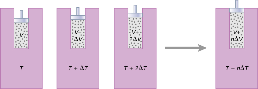
The change in entropy of a system for an arbitrary, reversible transition for which the temperature is not necessarily constant is defined by modifying \(\Delta S = Q/T\). Imagine a system making a transition from state A to B in small, discrete steps. The temperatures associated with these states are \(T_A\) and \(T_B\), respectively. During each step of the transition, the system exchanges heat \(\Delta Q_i\) reversibly at a temperature \(T_i\). This can be accomplished experimentally by placing the system in thermal contact with a large number of heat reservoirs of varying temperatures, \(T_i\), as illustrated in Figure \(\PageIndex{1}\). The change in entropy for each step is \(\Delta S_i = Q_i/T_i\). The net change in entropy of the system for the transition is
\[\Delta S = S_B - S_A = \sum_i \Delta S_i = \sum_i \dfrac{\Delta Q_i}{T_i}. \nonumber \]
We now take the limit as \(\Delta Q_i \rightarrow 0\), and the number of steps approaches infinity. Then, replacing the summation by an integral, we obtain
\[\Delta S = S_B - S_A = \int_A^B \dfrac{dQ}{T}, \label{eq5} \]
where the integral is taken between the initial state A and the final state B. This equation is valid only if the transition from A to B is reversible.

As an example, let us determine the net entropy change of a reversible engine while it undergoes a single Carnot cycle. In the adiabatic steps 2 and 4 of the cycle shown in Figure \(\PageIndex{1}\), no heat exchange takes place, so \(\Delta S_2 = \Delta S_4 = \int dQ/T = 0\). In step 1, the engine absorbs heat \(Q_h\) at a temperature \(T_h\), so its entropy change is \(\Delta S_1 = Q_h/T_h\). Similarly, in step 3, \(\Delta S_3 = -Q_c/T_c\). The net entropy change of the engine in one cycle of operation is then
\[\Delta S_E = \Delta S_1 + \Delta S_2 + \Delta S_3 + \Delta S_4 = \dfrac{Q_h}{T_h} - \dfrac{Q_c}{T_c}. \nonumber \]
However, we know that for a Carnot engine,
\[\dfrac{Q_h}{T_h} = \dfrac{Q_c}{T_c}, \nonumber \]
so
\[\Delta S_E = 0. \nonumber \]
There is no net change in the entropy of the Carnot engine over a complete cycle. Although this result was obtained for a particular case, its validity can be shown to be far more general: There is no net change in the entropy of a system undergoing any complete reversible cyclic process. Mathematically, we write this statement as
\[\oint dS = \oint \dfrac{dQ}{T} = 0 \label{eq10} \]
where \(\oint\) represents the integral over a closed reversible path.
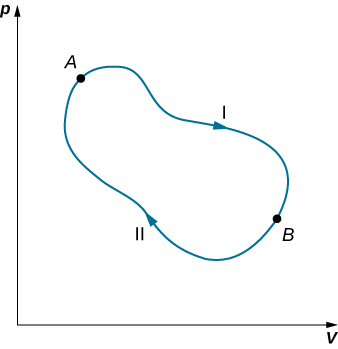
We can use Equation \ref{eq10} to show that the entropy change of a system undergoing a reversible process between two given states is path independent. An arbitrary, closed path for a reversible cycle that passes through the states A and B is shown in Figure \(\PageIndex{2}\). From Equation \ref{eq10}, we know that \(\oint dS = 0\) for this closed path. We may split this integral into two segments, one along I, which leads from A to B, the other along II, which leads from B to A. Then
\[\left[\int_A^BdS\right]_I + \left[\int_B^A dS\right]_{II} = 0 \nonumber \]
Since the process is reversible,
\[\left[\int_A^B dS\right] = \left[\int_A^B dS\right] \nonumber \]

Hence, the entropy change in going from A to B is the same for paths I and II. Since paths I and II are arbitrary, reversible paths, the entropy change in a transition between two equilibrium states is the same for all the reversible processes joining these states. Entropy, like internal energy, is therefore a state function.
What happens if the process is irreversible? When the process is irreversible, we expect the entropy of a closed system, or the system and its environment (the universe), to increase. Therefore we can rewrite this expression as
\[\Delta S \geq 0,\nonumber \]
where \(S\) is the total entropy of the closed system or the entire universe, and the equal sign is for a reversible process. The fact is the entropy statement of the second law of thermodynamics:
The entropy of a closed system and the entire universe never decreases.
We can show that this statement is consistent with the Kelvin statement, the Clausius statement, and the Carnot principle.
Determine the entropy change of an object of mass m and specific heat c that is cooled rapidly (and irreversibly) at constant pressure from \(T_h\) to \(T_c\).
Strategy
The process is clearly stated as an irreversible process; therefore, we cannot simply calculate the entropy change from the actual process. However, because entropy of a system is a function of state, we can imagine a reversible process that starts from the same initial state and ends at the given final state. Then, the entropy change of the system is given by Equation \ref{eq5}, \(\Delta S = \int_A^B dQ/T\).
Solution
To replace this rapid cooling with a process that proceeds reversibly, we imagine that the hot object is put into thermal contact with successively cooler heat reservoirs whose temperatures range from \(T_h\) to \(T_c\). Throughout the substitute transition, the object loses infinitesimal amounts of heat \(dQ\), so we have
\[\Delta S = \int_{T_h}^{T_c} \dfrac{dQ}{T}. \nonumber \]
From the definition of heat capacity, an infinitesimal exchange \(dQ\) for the object is related to its temperature change \(dT\) by
\[dQ = m~c~dT. \nonumber \]
Substituting this \(dQ\) into the expression for \(\Delta S\) we obtain the entropy change of the object as it is cooled at constant pressure from \(T_h\) to \(T_c\):
\[\Delta S = \int_{T_h}^{T_c} \dfrac{mcdT}{T} = mcln\dfrac{T_c}{T_h}. \nonumber \]
Note that \(\Delta S < 0\) here because \(T_c > T_h\). In other words, the object has lost some entropy. But if we count whatever is used to remove the heat from the object, we would still end up with \(S_{universe} > 0\) because the process is irreversible.
Significance
If the temperature changes during the heat flow, you must keep it inside the integral to solve for the change in entropy. If, however, the temperature is constant, you can simply calculate the entropy change as the heat flow divided by the temperature.
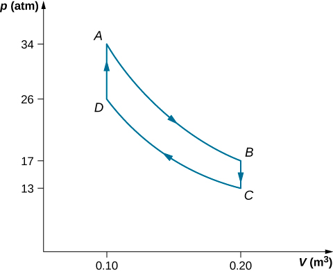
The steps of a reversible Stirling engine are as follows. For this problem, we will use 0.0010 mol of a monatomic gas that starts at a temperature of \(133^oC\) and a volume of \(0.10 m^3\) which will be called point A. Then it goes through the following steps:
- Step AB: isothermal expansion at \(33^oC\) from \(0.20 \, m^3\) to \(0.10 \, m^3\)
- Step BC: isochoric cooling to \(33^oC\)
- Step CD: isothermal compression at \(33^oC\) from \(0.20 \, m^3\) to \(0.10 \, m^3\)
- Step DA: isochoric heating back to \(133^oC\) and \(0.10 \, m^3\)
(a) Draw the pV diagram for the Stirling engine with proper labels.
(b) Fill in the following table.
| Step | W (J) | Q (J) | \(\Delta S\) (J/K) |
|---|---|---|---|
| Step AB | |||
| Step BC | |||
| Step CD | |||
| Step DA | |||
| Complete cycle |
(c) How does the efficiency of the Stirling engine compare to the Carnot engine working within the same two heat reservoirs?
Strategy
Using the ideal gas law, calculate the pressure at each point so that they can be labeled on the pV diagram. Isothermal work is calculated using \(W = nRT \, ln\left(\frac{V_2}{V_1}\right)\), and an isochoric process has no work done. The heat flow is calculated from the first law of thermodynamics, \(Q = \Delta E_{int} - W\) where \(\Delta E_{int} = \frac{3}{2}nR\Delta T\) for monatomic gasses. Isothermal steps have a change in entropy of Q/T, whereas isochoric steps have \(\Delta S = \frac{3}{2}n R \, ln \left(\frac{T_2}{T_1} \right)\). The efficiency of a heat engine is calculated by using \(e_{Stir} = W/Q_h\).
Solution
- The graph is shown below.

- The completed table is shown below.
Step W (J) Q (J) \(\Delta S\) (J/K) Step AB Isotherm 2.3 2.3 0.0057 Step BC Isochoric 0 –1.2 0.0035 Step CD Isotherm –1.8 –1.8 –0.0059 Step DA Isochoric 0 1.2 –0.0035 Complete cycle 0.5 0.5 ~ 0 - The efficiency of the Stirling heat engine is \[e_{Stir} = W/Q_h = (Q_{AB} + Q_{CD})/(Q_{AB} + Q{DA}) = 0.5/4.5 = 0.11. \nonumber \]
If this were a Carnot engine operating between the same heat reservoirs, its efficiency would be
\[e_{Car} = 1 - \left(\dfrac{T_c}{T_h} \right) = 0.25 \nonumber \]
Therefore, the Carnot engine would have a greater efficiency than the Stirling engine.
Significance
In the early days of steam engines, accidents would occur due to the high pressure of the steam in the boiler. Robert Stirling developed an engine in 1816 that did not use steam and therefore was safer. The Stirling engine was commonly used in the nineteenth century, but developments in steam and internal combustion engines have made it difficult to broaden the use of the Stirling engine.
The Stirling engine uses compressed air as the working substance, which passes back and forth between two chambers with a porous plug, called the regenerator, which is made of material that does not conduct heat as well. In two of the steps, pistons in the two chambers move in phase.


