12.6: Advanced Topics
- Page ID
- 22279
Chain of Masses Coupled with Spring- Dispersion, and Long-Wavelength Limit
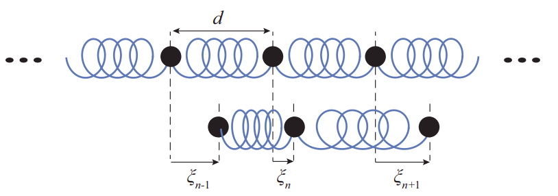
Consider a model of an extended elastic medium in which, for simplicity, we separate the two main medium properties, inertia and elasticity, by describing it as a chain of point-like masses (particles) connected by massless springs, as in Figure \(\PageIndex{1}\) below. I will show you here how one can get “ideal” wave behavior in this system, provided we work in the “long-wavelength” limit, that is to say, we consider only waves whose wavelength is much greater than the average distance between neighboring masses.

In the figure above I have explicitly shown the \(n\)-th mass and the two springs that push and/or pull on it, both in equilibrium (top drawing) and when the chain is in motion (bottom). In the latter case, the length of the springs depends on the relative displacements of all three masses shown. Specifically, the length of the spring on the left is \(d+\xi_n −\xi_{n−1}\), where \(d\) is the distance between the masses in equilibrium, and the length of the spring on the right is \(d + \xi_{n+1} − \xi_n\). If the left spring is stretched (length greater than \(d\)) it will pull to the left on the \(n\)-th mass, and, conversely, if the right spring is stretched (length greater than \(d\)) it will pull to the right on the \(n\)-th mass. So, if all the springs have the same constant \(k\), the force equation \(F = ma\) for mass \(n\) is
\[ m a_{n}=-k\left(\xi_{n}-\xi_{n-1}\right)+k\left(\xi_{n+1}-\xi_{n}\right) \label{eq:12.20} \]
which we can rewrite as
\[ m \frac{d^{2} \xi_{n}}{d t^{2}}=k \xi_{n-1}-2 k \xi_{n}+k \xi_{n+1} \label{eq:12.21} .\]
Now let us try to see if we can get a sinusoidal solution to this system of differential equations. By analogy with Equation (12.1.3) let
\[ \xi_{n}(t)=A \sin \left[2 \pi\left(\frac{x_{n}}{\lambda}-f t\right)\right] \nonumber \]
where \(x_n = nd\) is the equilibrium position of the \(n\)-th mass. Then for each of the three masses considered, we have
\begin{align}
\xi_{n-1}(t) &=A \sin [2 \pi((n-1) d / \lambda-f t)]=A \sin [2 \pi(n d / \lambda-f t)-2 \pi d / \lambda] \nonumber \\
\xi_{n}(t) &=A \sin [2 \pi(n d / \lambda-f t)] \nonumber \\
\xi_{n+1}(t) &=A \sin [2 \pi((n+1) d / \lambda-f t)]=A \sin [2 \pi(n d / \lambda-f t)+2 \pi d / \lambda] \label{eq:12.22}
\end{align}
We want to substitute all this in Equation (\ref{eq:12.21}). We can use the trigonometric identity \(\sin(a − b) + \sin(a + b) = 2 \sin a \cos b\) to simplify \(\xi_{n−1} + \xi_{n+1}\):
\[ \xi_{n-1}+\xi_{n+1}=2 A \sin \left[2 \pi\left(\frac{n d}{\lambda}-f t\right)\right] \cos \left(\frac{2 \pi d}{\lambda}\right) \label{eq:12.23} \]
then use \(1 − \cos x = 2 \sin ^2 (x/2)\) to yield
\[ k \xi_{n-1}-2 k \xi_{n}+k \xi_{n+1}=-4 k A \sin ^{2}\left(\frac{\pi d}{\lambda}\right) \sin \left[2 \pi\left(\frac{n d}{\lambda}-f t\right)\right]=-4 k \sin ^{2}\left(\frac{\pi d}{\lambda}\right) \xi_{n} \label{eq:12.24} \]
It is clear now that Equation (\ref{eq:12.21}) will be satisfied provided the following condition holds:
\[ m(2 \pi f)^{2}=4 k \sin ^{2}\left(\frac{\pi d}{\lambda}\right) \label{eq:12.25} .\]
Or, taking the square root and simplifying,
\[ f=\frac{1}{\pi} \sqrt{\frac{k}{m}} \sin \left(\frac{\pi d}{\lambda}\right) \label{eq:12.26} .\]
This is clearly a more complicated relation between \(f\) and \(\lambda\) than just Equation (12.1.4). However, since we can argue that Equation (12.1.4) must always hold for a sinusoidal wave, what we have actually found is that the chain of masses and springs in Figure \(\PageIndex{1}\) will support a sinusoidal wave provided the wave velocity depends on the wavelength as required by Eqs. (12.1.4) and (\ref{eq:12.26}):
\[ c=\lambda f=\sqrt{\frac{k}{m}} \frac{\lambda}{\pi} \sin \left(\frac{\pi d}{\lambda}\right) \label{eq:12.27} .\]
This is an instance of the phenomenon called dispersion: sinusoidal waves of different frequencies (or wavelengths) have different velocities. One thing that happens in the presence of dispersion is that, although a single (infinite), sinusoidal wave can travel without changing its shape (provided \(f\) and \(\lambda\) satisfy Equation (\ref{eq:12.26})), a general pulse will be distorted as it propagates through the medium, often severely so.
In the long wavelength limit, however, the dispersion in this model disappears. We can see this as follows. In that limit, \(\lambda \gg d\) (the wavelength is much greater than the distance between the masses), and therefore \(\pi d / \lambda \ll 1\); we can then make the small-angle approximation in Equation (\ref{eq:12.27}), \(\sin (\pi d / \lambda) \simeq \pi d / \lambda\), and end up with
\[ c \simeq d \sqrt{\frac{k}{m}} \label{eq:12.28} .\]
This is of the general form \(\sqrt{\text { stiffness/inertia }}\) (as per Equation (12.1.10)). Basically, in the long-wavelength limit, the medium appears homogeneous to the wave—it cannot “tell” that it is a chain of discrete particles. When you consider that everything that looks homogeneous on a macroscopic scale is actually made of discrete atoms or molecules at the microscopic level, you can see that this model is perhaps not as artificial as it might seem, and that in general you should, in fact, expect some kind of dispersion to occur in any medium, at sufficiently small wavelengths.


