1.2: Small Oscillations and Linearity

A system with one degree of freedom is linear if its equation of motion is a linear function of the coordinate, $x$, that specifies the system’s configuration. In other words, the equation of motion must be a sum of terms each of which contains at most one power of $x$. The equation of motion involves a second derivative, but no higher derivatives, so a linear equation of motion has the general form:

$$α\frac{d^2}{dt^2}x(t) + β\frac{d}{dt}x(t) + γx(t) = f(t)$$

If all of the terms involve exactly one power of x, the equation of motion is “homogeneous.” Equation (1) is not homogeneous because of the term on the right-hand side. The “inhomogeneous” term, f(t), represents an external force. The corresponding homogeneous equation would look like this:

$$α\frac{d^2}{dt^2}x(t) + β\frac{d}{dt}x(t) + γx(t) = 0$$

In general, $α$, $β$ and $γ$ as well as $f$ could be functions of $t$. However, that would break the time translation invariance that we will discuss in more detail below and make the system much more complicated. We will almost always assume that $α$, $β$ and $γ$ are constants. The equation of motion for the mass on a spring, $m\frac{d^2}{dt^2}x(t) = -Kx(t)$, is of this general form, but with β and f equal to zero. As we will see in chapter 2, we can include the effect of frictional forces by allowing nonzero β, and the effect of external forces by allowing nonzero f. The linearity of the equation of motion, (1), implies that if $x_1(t)$ is a solution for external force $f_1(t)$,

$$α\frac{d^2}{dt^2}x_1(t) + β\frac{d}{dt}x_1(t) + γx_1(t) = f_1(t)$$

and $x_2(t)$ is a solution for external force $f_2(t)$,

$$α\frac{d^2}{dt^2}x_2(t) + β\frac{d}{dt}x_2(t) + γx_2(t) = f_2(t)$$

then the sum,

$$x_{12}(t) = Ax_1(t) + Bx_2(t)$$

for constants A and B is a solution for external force $Af_1 + Bf_2$,

$$α\frac{d^2}{dt^2}x_{12}(t) + β\frac{d}{dt}x_{12}(t) + γx_{12}(t) = Af_1(t) + Bf_2(t)$$

The sum $x_{12}(t)$ is called a “linear combination” of the two solutions, $x_1(t)$ and $x_2(t)$. In the case of “free” motion, which means motion with no external force, if $x_1(t)$ and $x_2(t)$ are solutions, then the sum, $A x_1(t) + B x_2(t)$ is also a solution.

The most general solution to any of these equations involves two constants that must be fixed by the initial conditions, for example, the initial position and velocity of the particle, as in $x(t) = x(0)cos(ωt) + \frac{1}{ω}x'(0)sin(ωt)$. It follows from (6) that we can always write the most general solution for any external force, f(t), as a sum of the “general solution” to the homogeneous equation, (2), and any “particular” solution to (1).

No system is exactly linear. “Linearity” is never exactly “true.” Nevertheless, the idea of linearity is extremely important, because it is a useful approximation in a very large number of systems, for a very good physical reason. In almost any system in which the properties are smooth functions of the positions of the parts, the small displacements from equilibrium produce approximately linear restoring forces. The difference between something that is “true” and something that is a useful approximation is the essential difference between physics and mathematics. In the real world, the questions are much too interesting to have answers that are exact. If you can understand the answer in a well-defined approximation, you have learned something important.

To see the generic nature of linearity, consider a particle moving on the x-axis with potential energy, $V (x)$. The force on the particle at the point, $x$, is minus the derivative of the potential energy,

$$F = -\frac{d}{dx}V(x)$$

A force that can be derived from a potential energy in this way is called a “conservative” force. At a point of equilibrium, $x_0$, the force vanishes, and therefore the derivative of the potential energy vanishes:

$$F = -\frac{d}{dx}V(x)|_{x=x_0} = -V'(v_o) = 0$$

We can describe the small oscillations of the system about equilibrium most simply if we redefine the origin so that $x_0 = 0$. Then the displacement from equilibrium is the coordinate x. We can expand the force in a Taylor series:

$$F(x) = -V'(x) = -V'(0) - xV''(0) - \frac{1}{2}x^2V'''(0) + ...$$

The first term in (9) vanishes because this system is in equilibrium at x = 0, from (8). The second term looks like Hooke’s law with

$$K = V''(0)$$

The equilibrium is stable if the second derivative of the potential energy is positive, so that $x = 0$ is a local minimum of the potential energy. The important point is that for sufficiently small x, the third term in (9), and all subsequent terms will be much smaller than the second. The third term is negligible if

$$|xV'''(0)| <<V''(0)$$

Typically, each extra derivative will bring with it a factor of 1/L, where L is the distance over which the potential energy changes by a large fraction. Then (11) becomes

$$x<<L$$

There are only two ways that a force derived from a potential energy can fail to be approximately linear for sufficiently small oscillations about stable equilibrium:

1. If the potential is not smooth so that the first or second derivative of the potential is not well defined at the equilibrium point, then we cannot do a Taylor expansion and the argument of (9) does not work. We will give an example of this kind at the end of this chapter.

2. Even if the derivatives exist at the equilibrium point, x = 0, it may happen that $V''(0) = 0$. In this case, to have a stable equilibrium, we must have $V'''(0) = 0$ as well, otherwise a small displacement in one direction or the other would grow with time. Then the next term in the Taylor expansion dominates at small $x$, giving a force proportional to $x^3$.

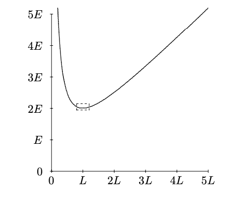
Figure 1.2: The potential energy of (13)

Both of these exceptional cases are very rare in nature. Usually, the potential energy is a smooth function of the displacement and there is no reason for V''(0) to vanish. The generic situation is that small oscillations about stable equilibrium are linear.

An example may be helpful. Almost any potential energy function with a point of stable equilibrium will do, so long as it is smooth. For example, consider the following potential energy

$$V(x) = E(\frac{L}{x} + \frac{x}{L})$$

This is shown in figure 1.2. The minimum (at least for positive $x$) occurs at $x=L$, so we first redefine $x= X + L$, so that

$$V(X) = E(\frac{L}{X+L} + \frac{X+L}{L})$$

The corresponding force is

$$F(X) = E(\frac{L}{(X+L)^2} - \frac{1}{L})$$

we can look near $X = 0$ and expand in a Taylor Series:

$$F(X) = -2\frac{E}{L}(\frac{X}{L}) + 3\frac{E}{L}(\frac{X}{L})^2 + ...$$

Now, the ratio of the first nonlinear term to the linear term is

$$\frac{3X}{2L}$$

which is small if X<<L.

In other words, the closer you are to the equilibrium point, the closer the actual potential energy is to the parabola that we would expect from the potential energy for a linear, Hooke’s law force. You can see this graphically by blowing up a small region around the equilibrium point. In figure 1.3, the dotted rectangle in figure 1.2 has been blown up into a square. Note that it looks much more like a parabola than figure 1.3. If we repeated the procedure and again expanded a small region about the equilibrium point, you would not be able to detect the cubic term by eye.

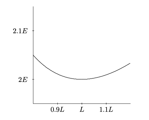
Figure 1.3: The small dashed rectangle in figure 1.2 expanded

Often, the linear approximation is even better, because the term of order $x^2$ vanishes by symmetry. For example, when the system is symmetrical about x = 0, so that $V(x) = V(-x)$, the order $x^3$ term (and all $x^n$ for $n$ odd) in the potential energy vanishes, and then there is no order $x^2$ term in the force.

For a typical spring, linearity (Hooke’s law) is an excellent approximation for small displacements. However, there are always nonlinear terms that become important if the displacements are large enough. Usually, in this book we will simply stick to small oscillations and assume that our systems are linear. However, you should not conclude that the subject of nonlinear systems is not interesting. In fact, it is a very active area of current research in physics.