9.3: Transfer Matrices

Masses on a String

Next consider the reflection and transmission from two masses on a string, as in Figure $9.5$. Now translation invariance and the boundary condition at $x = \infty$ imply that $$\psi(x, t)=A e^{i k x} e^{-i \omega t}+R A e^{-i k x} e^{-i \omega t} \text { for } x \leq 0 ,$$

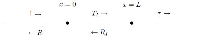
Figure $9.5$: Two masses on a string.

$$\psi(x, t)=T_{I} A e^{i k x} e^{-i \omega t}+R_{I} A e^{-i k x} e^{-i \omega t} \text { for } 0 \leq x \leq L ,$$

$$\psi(x, t)=\tau A e^{i k x} e^{-i \omega t} \text { for } x \geq L .$$

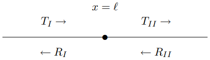
Figure $9.6$: The general scattering problem from a mass on a string.

We could solve this problem in the same way, simply imposing boundary conditions twice, at $x = 0$ and at $x = L$, but there is a systematic way of doing this that is very useful. Consider first the general scattering problem from a single mass at $x = \ell$, with both incoming and outgoing waves on both sides, as shown in Figure $9.6$. This is the most general possible thing that can happen in scattering from a single mass, and we will be able to use the result to do much more complicated problems without any additional work. The general solution has the form $$\psi(x, t)=T_{I} A e^{i k x} e^{-i \omega t}+R_{I} A e^{-i k x} e^{-i \omega t} \text { for } x \leq \ell ,$$

$$\psi(x, t)=T_{I I} A e^{i k x} e^{-i \omega t}+R_{I I} A e^{-i k x} e^{-i \omega t} \text { for } x \geq \ell .$$

The boundary conditions are continuity — $$T_{I} e^{i k \ell}+R_{I} e^{-i k \ell}=T_{I I} e^{i k \ell}+R_{I I} e^{-i k \ell}$$

and $F = ma$ — $$\begin{gathered} T\left(\left.\frac{\partial}{\partial x} \psi(x, t)\right|_{x=\ell^{+}}-\left.\frac{\partial}{\partial x} \psi(x, t)\right|_{x=\ell^{-}}\right) \\ =m \frac{\partial^{2}}{\partial t^{2}} \psi(\ell, t) \end{gathered}$$

or $$\begin{aligned} &i k T\left(\left(T_{I I}-T_{I}\right) e^{i k \ell}+\left(R_{I}-R_{I I}\right) e^{-i k \ell}\right) \\ &=-m \omega^{2}\left(T_{I I} e^{i k \ell}+R_{I I} e^{-i k \ell}\right) . \end{aligned}$$

Solving for $T_{I}$ and $R_{I}$ gives $$\begin{aligned} &T_{I}=\frac{1}{2}\left[(2-i \epsilon) T_{I I}-i \epsilon R_{I I} e^{-2 i k \ell}\right] , \\ &R_{I}=\frac{1}{2}\left[(2+i \epsilon) R_{I I}+i \epsilon T_{I I} e^{2 i k \ell}\right] . \end{aligned}$$

The important point is that because of linearity, the result (9.69) can be written in matrix form: $$\left(\begin{array}{l} T_{I} \\ R_{I} \end{array}\right)=d(\ell)\left(\begin{array}{l} T_{I I} \\ R_{I I} \end{array}\right)$$

where the matrix $d(\ell)$ $$d(\ell)=\frac{1}{2}\left(\begin{array}{cc} (2-i \epsilon) & -i \epsilon e^{-2 i k \ell} \\ i \epsilon e^{2 i k \ell} & (2+i \epsilon) \end{array}\right) .$$

The matrix, $d(\ell)$, is a “transfer matrix.” It allows us to get from the amplitudes in one region to those in the next by just doing a matrix multiplication. We can use this to solve the two mass problem without any further calculation except a matrix multiplication. Comparing the general result, (9.70), with the two mass problem, Figure $9.5$, we see immediately that $$\left(\begin{array}{l} 1 \\ R \end{array}\right)=d(0)\left(\begin{array}{l} T_{I} \\ R_{I} \end{array}\right) ,$$

and $$\left(\begin{array}{c} T_{I} \\ R_{I} \end{array}\right)=d(L)\left(\begin{array}{l} \tau \\ 0 \end{array}\right) .$$

Thus $$\left(\begin{array}{l} 1 \\ R \end{array}\right)=d(0) d(L)\left(\begin{array}{l} \tau \\ 0 \end{array}\right) .$$

Doing the matrix multiplication, $$\begin{gathered} d(0) d(L)=\frac{1}{4} \\ \left(\begin{array}{cc} (2-i \epsilon)^{2}+\epsilon^{2} e^{2 i k L} & -i \epsilon\left((2-i \epsilon) e^{-2 i k L}+(2+i \epsilon)\right) \\ i \epsilon\left((2-i \epsilon)+(2+i \epsilon) e^{2 i k L}\right) & (2+i \epsilon)^{2}+\epsilon^{2} e^{-2 i k L} \end{array}\right) . \end{gathered}$$

So $$\begin{gathered} \tau=\frac{4}{(2-i \epsilon)^{2}+\epsilon^{2} e^{2 i k L}} , \\ R=i \epsilon\left((2-i \epsilon)+(2+i \epsilon) e^{2 i k L}\right) \frac{\tau}{4} . \end{gathered}$$

Note that the reflection and transmission shows interesting resonance structure. For example, the reflection vanishes for $$e^{2 i k L}=-\frac{2-i \epsilon}{2+i \epsilon} .$$

In Figure $9.7$, $|\tau|$ and $|R|$ are plotted versus $\epsilon$ for $k L=0.5$.

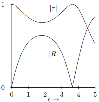
Figure $9.7$: $|\tau|$ and $|R|$ plotted versus $\epsilon$ for two masses on a string.

$k$ Changes Region

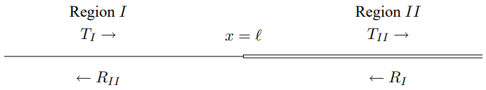
Figure $9.8$: The general scattering problem for a change of $k$.

Let us return to the simple example at the beginning of the chapter of a boundary between two regions of string with different values of $k$. This is a very important example because its general features are characteristic of many important physical systems. For example, when a light-wave encounters a transparent medium, the $k$ value changes. That situation is somewhat more complicated because of the three-dimensional nature of light waves and because of polarization. However the analogy between (9.59) and (9.9) and (9.10) means that we can take over the discussion of of the string directly to electromagnetic waves reflecting from a dielectric boundary perpendicular to the direction of the wave. In this section, we apply the general method of transfer matrices discussed in the previous section to this important example. Thus we consider the situation shown in Figure $9.8$. where the waves have the form $$\psi(x, t)=A e^{-i \omega t}\left(T_{I} e^{i k_{1} x}+R_{I} e^{-i k_{1} x}\right) \text { in } I ,$$

$$\psi(x, t)=A e^{-i \omega t}\left(T_{I I} e^{i k_{2} x}+R_{I I} e^{-i k_{2} x}\right) \text { in } I I .$$

Then as in (9.9) and (9.10), the boundary conditions are that $\psi$ is continuous at $x = \ell$, which implies $$T_{I} e^{i k_{1} \ell}+R_{I} e^{-i k_{1} \ell}=T_{I I} e^{i k_{2} \ell}+R_{I I} e^{-i k_{2} \ell} ,$$

and that the slope, $\partial \psi / \partial x$ is continuous at $x = \ell$, which implies $$i k_{1}\left(T_{I} e^{i k_{1} \ell}-R_{I} e^{-i k_{1} \ell}\right)=i k_{2}\left(T_{I I} e^{i k_{2} \ell}-R_{I I} e^{-i k_{2} \ell}\right) .$$

Solving the simultaneous linear equations, (9.80) and (9.81), for $T_{I}$ and $R_{I}$ and expressing the result in matrix form, we find $$\left(\begin{array}{c} T_{I} \\ R_{I} \end{array}\right)=d\left(k_{1}, k_{2}, \ell\right)\left(\begin{array}{c} T_{I I} \\ R_{I I} \end{array}\right) ,$$

where $$d\left(k_{1}, k_{2}, \ell\right)=\frac{1}{2}\left(\begin{array}{ll} \left(1+\frac{k_{2}}{k_{1}}\right) & e^{i k_{2} \ell-i k_{1} \ell} & \left(1-\frac{k_{2}}{k_{1}}\right) e^{-i k_{2} \ell-i k_{1} \ell} \\ \left(1-\frac{k_{2}}{k_{1}}\right) & e^{i k_{2} \ell+i k_{1} \ell} & \left(1+\frac{k_{2}}{k_{1}}\right) e^{-i k_{2} \ell+i k_{1} \ell} \end{array}\right) .$$

(9.82) is a very general result because $k_{1}$, $k_{2}$ and $\ell$ can be anything. Note that the relation is symmetrical: $$\left(\begin{array}{c} \bar{T}_{I I} \\ R_{I I} \end{array}\right)=d\left(k_{2}, k_{1}, \ell\right)\left(\begin{array}{c} T_{I} \\ R_{I} \end{array}\right) .$$

In matrix language, that implies that $$d\left(k_{2}, k_{1}, \ell\right) d\left(k_{1}, k_{2}, \ell\right)=I .$$

It is also useful to use the properties of matrix multiplication to rewrite (9.83) in the following form: $$d\left(k_{1}, k_{2}, \ell\right)=b\left(k_{1}, \ell\right)^{-1} \tau\left(k_{1}, k_{2}\right) b\left(k_{2}, \ell\right) ,$$

where $$b(k, \ell)=\left(\begin{array}{cc} e^{i k \ell} & 0 \\ 0 & e^{-i k \ell} \end{array}\right) ,$$

and $$\tau\left(k_{1}, k_{2}\right)=d\left(k_{1}, k_{2}, 0\right)=\frac{1}{2}\left(\begin{array}{ll} \left(1+\frac{k_{2}}{k_{1}}\right) & \left(1-\frac{k_{2}}{k_{1}}\right) \\ \left(1-\frac{k_{2}}{k_{1}}\right) & \left(1+\frac{k_{2}}{k_{1}}\right) \end{array}\right) .$$

You will see the utility of this in the computer problem, (9.6).

Reflection from a Thin Film

Figure $9.9$: Reflection from a thin film.

Consider the situation shown in Figure $9.9$. where the wave numbers are $k_{1}$ for $x \leq 0$, $k_{2}$ for $0 \leq x \leq L$ and $k_{3}$ for $x \geq L$. As usual, translation invariance plus the boundary condition at infinity (that the incoming wave in $I$ has amplitude, $A$, and that there is only an outgoing wave in $III$) implies $$\begin{gathered} \psi(x, t)=A e^{-i \omega t}\left(e^{i k_{1} x}+R e^{-i k_{1} x}\right) \quad \text { for } x \leq 0 \\ \psi(x, t)=A e^{-i \omega t}\left(T_{I I} e^{i k_{2} x}+R_{I I} e^{-i k_{2} x}\right) \text { for } 0 \leq x \leq L, \\ \psi(x, t)=\tau A e^{-i \omega t} e^{i k_{3} x} \text { for } L \leq x . \end{gathered}$$

Then we know from the results of the previous section that $$\left(\begin{array}{l} 1 \\ R \end{array}\right)=d\left(k_{1}, k_{2}, 0\right)\left(\begin{array}{l} T_{I I} \\ R_{I I} \end{array}\right)$$

and $$\left(\begin{array}{c} T_{I I} \\ R_{I I} \end{array}\right)=d\left(k_{2}, k_{3}, L\right)\left(\begin{array}{l} \tau \\ 0 \end{array}\right)$$

and therefore $$\begin{gathered} \left(\begin{array}{c} 1 \\ R \end{array}\right)=d\left(k_{1}, k_{2}, 0\right) d\left(k_{2}, k_{3}, L\right)\left(\begin{array}{c} \tau \\ 0 \end{array}\right) . \\ d\left(k_{1}, k_{2}, 0\right) d\left(k_{2}, k_{3}, L\right) \\ =b\left(k_{1}, 0\right)^{-1} \tau\left(k_{1}, k_{2}\right) b\left(k_{2}, 0\right) b\left(k_{2}, L\right)^{-1} \tau\left(k_{2}, k_{3}\right) b\left(k_{3}, L\right) \end{gathered}$$

Often we are interested in the situation $k_{3} = k_{1}$, that describes a film (in one-dimension, a film is just a region in $x$) in an otherwise homogeneous medium. This is then a one-dimensional analog of the reflection of light from a soap bubble. Then the transfer matrix looks like $$\begin{gathered} \frac{1}{4}\left(\begin{array}{ll} \left(1+\frac{k_{2}}{k_{1}}\right) & \left(1-\frac{k_{2}}{k_{1}}\right) \\ \left(1-\frac{k_{2}}{k_{1}}\right) & \left(1+\frac{k_{2}}{k_{1}}\right) \end{array}\right)\left(\begin{array}{cc} e^{-i k_{2} L} & 0 \\ 0 & e^{i k_{2} L} \end{array}\right) \\ \left(\begin{array}{ll} \left(1+\frac{k_{1}}{k_{2}}\right) & \left(1-\frac{k_{1}}{k_{2}}\right) \\ \left(1-\frac{k_{1}}{k_{2}}\right) & \left(1+\frac{k_{1}}{k_{2}}\right) \end{array}\right)\left(\begin{array}{cc} e^{i k_{1} L} & 0 \\ 0 & e^{-i k_{1} L} \end{array}\right) \end{gathered}$$

Thus $$1=\left(\cos k_{2} L-i \frac{k_{1}^{2}+k_{2}^{2}}{2 k_{1} k_{2}} \sin k_{2} L\right) e^{i k_{1} L} \tau$$

and $$R=-\left(i \frac{k_{1}^{2}-k_{2}^{2}}{2 k_{1} k_{2}} \sin k_{2} L\right) e^{i k_{1} L} \tau$$

or $$\tau=\left(\cos k_{2} L-i \frac{k_{1}^{2}+k_{2}^{2}}{2 k_{1} k_{2}} \sin k_{2} L\right)^{-1} e^{-i k_{1} L}$$

and $$R=-\left(i \frac{k_{1}^{2}-k_{2}^{2}}{2 k_{1} k_{2}} \sin k_{2} L\right)\left(\cos k_{2} L-i \frac{k_{1}^{2}+k_{2}^{2}}{2 k_{1} k_{2}} \sin k_{2} L\right)^{-1} .$$

Here we see the phenomenon of resonant transmission. The wave does not get reflected at all if the thickness of the film is an integral or half-integral number of wavelengths. Note, also, that when $k_{2} \rightarrow k_{1}$, $\tau \rightarrow 1$ and $R \rightarrow 0$ as they should, because in this limit there is no boundary.

The reflection in (9.98) varies rapidly with $k_{2}$, as shown Figure $9.10$, where we plot the intensity of the reflected wave versus $k_{2}$ for fixed ratio $k_{1} / k_{2} = 3$. It is this rapid variation of the intensity of reflected light as a function of wavelength that is responsible for the familiar color patterns on thin films like soap bubbles and oil slicks.

Figure $9.10$: Graph of $|R|^{2}$ versus $k_{2}$ for $k_{1} / k_{2} = 3$.

Nonreflective Coating

We will not work out the general case of $k_{1} \neq k_{3}$, simply because the algebra is a mess. However, one important special case is worth noting. Suppose that you have a boundary between media in which the wave number of your traveling wave are $k_{1}$ and $k_{3}$. Normally, you find reflection at the boundary. The question is, can you add an intermediate film layer with wave number $k_{2}$, that eliminates all reflection? The answer is yes. First you must adjust the wave number in the film to be the geometric mean of $k_{1}$ and $k_{3}$, so that $$\frac{k_{2}}{k_{1}}=\frac{k_{3}}{k_{2}} .$$

Then the transfer matrix becomes $$\begin{aligned} &\frac{1}{4}\left(\begin{array}{ll} \left(1+\frac{k_{2}}{k_{1}}\right) & \left(1-\frac{k_{2}}{k_{1}}\right) \\ \left(1-\frac{k_{2}}{k_{1}}\right) & \left(1+\frac{k_{2}}{k_{1}}\right) \end{array}\right)\left(\begin{array}{cc} e^{-i k_{2} L} & 0 \\ 0 & e^{i k_{2} L} \end{array}\right) \\ &\left(\begin{array}{cc} \left(1+\frac{k_{2}}{k_{1}}\right) & \left(1-\frac{k_{2}}{k_{1}}\right) \\ \left(1-\frac{k_{2}}{k_{1}}\right) & \left(1+\frac{k_{2}}{k_{1}}\right) \end{array}\right)\left(\begin{array}{cc} e^{i k_{3} L} & 0 \\ 0 & e^{-i k_{3} L} \end{array}\right) . \end{aligned}$$

It is easy to check that the reflection vanishes when there are a half-odd-integral number of wavelengths in the intermediate region, $$k_{2} L=(2 n+1) \frac{\pi}{2} .$$

In qualitative terms, the reflection vanishes because of a destructive interference between the reflected waves from the two boundaries. This has practical applications to nonreflective coatings for optical components.