9.4: Chapter Checklist

You should now be able to:

1. Analyze scattering problems by imposing boundary conditions and computing reflection and transmission coefficients;
2. Identify a wave with some reflection, and differentiate it from a pure traveling or standing wave;
3. Check energy conservation in scattering problems;
4. Analyze electromagnetic plane waves in a dielectric, and the reflection from a dielectric boundary;
5. *Use transfer matrices to simplify the analysis of scattering from more than one boundary.

Problems

9.1.

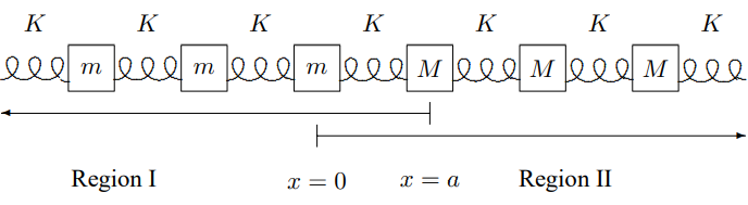
Shown above is the boundary between two semi-infinite systems. To the left, there are identical blocks of mass \(m\). To the right, there are identical blocks of mass \(M\). They are connected as shown by identical massless springs with spring constant \(K\), such that the equilibrium separation between neighboring blocks is \(a\). Consider the reflection of a traveling longitudinal wave from the boundary between these two regions. That is, assume that in region I there is an incident wave of amplitude \(A\) traveling to the right and a reflected wave traveling to the left. In a complex notation, the displacement of the mass with equilibrium position \(x\) is \[\psi(x, l)=A e^{-i(\omega t-k x)}+R A e^{-i(\omega t+k x)}\]

for \(x \leq a\). What is the relation between \(\omega\) and \(k\)?

In region II, there is only a transmitted wave: \[\psi(x, l)=A e^{-i(\omega t-k x)}+R A e^{-i(\omega t+k x)}\]

for \(x \geq 0\). What is the relation between \(\omega\) and \(k^{\prime}\)? Find the appropriate boundary conditions that allow you to relate \(\psi(x,t)\) in the two regions and solve for \(R\) (do not bother to simplify the complex number). Check your result by taking the limit of \(a\), \(m\) and \(M\) going to zero with \(m / a\) and \(M / a\) fixed and comparing with an appropriate continuous system.

9.2. An infinite line of coupled pendulums supports traveling waves, but it has no standing wave normal modes in which the displacement of the pendulums goes to zero at infinity. Consider, however, the system shown below:

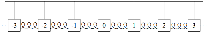
Here block 0 is free to slide longitudinally with no gravitational restoring force, only the coupling due to the springs. If the blocks have mass \(M\), the springs’ spring constant \(K\), the separation between neighboring blocks is \(a\), and the pendulums have length \(\ell\), find the frequency of the standing wave normal mode of the system in which the displacements are \(A e^{-\kappa x}\) for \(x \geq 0\) and \(A e^{\kappa x}\) for \(x \leq 0\). Hint: Consider the subsystem, \(-a \leq x \leq a\), as part of an infinite system with appropriate boundary conditions. Then you can get the answer directly from the dispersion relation.

9.3.

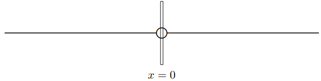
Consider a string with linear mass density \(\rho\), split into two pieces. The two halves are attached to a massless ring which slides vertically without friction on a rod at \(x = 0\). One of the two halves is stretched in the negative \(x\) direction with tension \(T\). The other is stretched in the positive \(x\) direction with tension \(T^{\prime}\). Note that the vertical rod is necessary to balance the horizontal forces on the massless ring from the two strings with different tensions.

Suppose that a traveling wave comes in from the negative \(x\) direction. Then the displacement of the strings in the two regions is \[\begin{gathered}
\psi(x, t)=A e^{i k x} e^{-i \omega t}+R A e^{-i k^{\prime} x} e^{-i \omega^{\prime} t} \text { for } x \leq 0 \\
\psi(x, t)=\tau A e^{i k^{\prime \prime} x} e^{-i \omega^{\prime \prime} t} \text { for } x \geq 0 .
\end{gathered}\]

1. Find k, k0 , ω0 , k00 and ω00 in terms of ω, T, T0 and ρ. Hint – this is easy!
2. Write down the two boundary conditions at x = 0 and find R and τ .

9.4. Consider traveling waves in an infinite system, part of which is shown below, for longitudinal (horizontal) motion of the blocks.

All the blocks have mass \(m\), except for block 0 which is massless. The springs are massless and have spring constant \(K\). The separation between neighboring blocks is \(a\). To the left of block 0, which we will take to be at \(x = 0\), there is an incoming and a reflected wave, so that the longitudinal displacement of the blocks for \(x \leq 0\) has the form \[A e^{i k x-i \omega t}+R A e^{-i k x-i \omega t} .\]

To the right of the massless block, there is a transmitted wave, so that the longitudinal displacement of the blocks for \(x \geq 0\) has the form \[T A e^{i k x-i \omega t} .\]

\(\omega\) and \(k\) are related by the dispersion relation \[\omega^{2}=\frac{4 K}{m} \sin ^{2} \frac{k a}{2} .\]

1. Explain the physics of the boundary conditions at \(x = 0\).
2. Find \(R\) and \(T\).

9.5. Consider a semi-infinite system of two kinds of massive string with different densities, shown below:

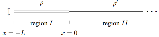
The density of the string in region \(I\) is \(\rho\) and in region \(II\) is \(\rho^{\prime}\). The tension in both strings is \(T\). Suppose that the end at \(x = −L\) is oscillated in the transverse direction with displacement \(\chi \sin \omega t\). This produces an outgoing wave (moving to the right) in region \(II\) with no incoming wave. Suppose that \(\omega=\frac{\pi}{2 L} \sqrt{\frac{T}{\rho}}\). Find the displacement at the point \(x = 0\) as a function of time.

9.6. If you are doing a reflection and transmission problem involving several different regions, and thus requiring several boundary conditions, the transfer matrix is very helpful. You saw this in the analysis of scattering from a thin film.

Your computer assignment is to extend this analysis to incorporate \(2 \pi\) such boundary conditions where n is some large integer. In particular, consider a continuous string with wave number \(k_{2}\) for \(L \leq x \leq 2 L, 3 L \leq x \leq 4 L\), \(\cdots\), and \((2 n-1) L \leq x \leq 2 n L\), and \(k_{1}\) elsewhere.

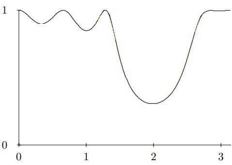
Figure \( 9.11\): \(n = 3\).

Take \(k_{1} = k\) and \(k_{2} = 2k\). Compute the amplitude for transmission of an incoming wave in this system as a function of \(L\) by doing the appropriate multiplication of \(2n\) matrices. To do this, you must program your computer to multiply complex matrices. Organize your program in an iterative way, so that you can change n easily. This will allow you to start out with small \(n\) and go to larger \(n\) only when you are sure that the program is working.

If possible, you should present the results in the form of a graph of the absolute value of the transmission coefficient versus \(kL\), for \(0 \leq L \leq \pi / 2 k\). As you go to higher \(n\), something interesting happens. The transmission coefficient drops nearly to zero in a region of \(L\) values. Even if you cannot produce a graph, you should be able to find the range of \(L\) for which the transmission goes to zero as \(n\) gets large.

Hint: For \(n = 3\), the result should look like the graph in Figure \( 9.11\).