13.4: Examples

Single Slit

Suppose \[f(x, y)=\left\{\begin{array}{l}
1 \text { for }-a \leq x \leq a \\
0 \text { for }|x|>a
\end{array}\right.\]

independent of \(y\). This is really a two-dimensional problem, because we can keep \(k_{y} = 0\) and ignore it (except for a factor of \(2\pi\), that we won’t worry about) by dropping the \(k_{y}\) integral from (13.19). (13.24) \[C\left(k_{x}, k_{y}\right)=\frac{1}{4 \pi^{2}} \int d x d y f(x, y) e^{-i\left(k_{x} x+k_{y} y\right)}\]

becomes (with the \(2\pi\) corrected to make it one-dimensional)⁷ \[\begin{gathered}
C\left(k_{x}\right)=\frac{1}{2 \pi} \int_{-\infty}^{\infty} d x f(x) e^{-i k_{x} x} \\
=\frac{1}{2 \pi} \int_{-a}^{a} d x e^{-i k_{x} x}=\left.\frac{1}{-2 i \pi k_{x}} e^{-i k_{x} x}\right|_{-a} ^{a}=\frac{\sin k_{x} a}{\pi k_{x}} .
\end{gathered}\]

Thus we expect that the intensity of the wave at large \(z\) is proportional to \(\left|C\left(k_{x}\right)\right|^{2}\), \[I(x, y) \propto \frac{\sin ^{2}\left(k_{x} a\right)}{k_{x}^{2}}\]

where \[\frac{x}{r}=\frac{k_{x}}{k}=\frac{k_{x}}{\omega / v}\]

or \[k_{x}=\frac{\omega}{v} \frac{x}{r}.\]

Thus if we measure the intensity of the diffracted beam, a distance \(r\) from the opening, the intensity goes as follows:⁸ \[I(x, y) \propto \frac{\sin ^{2}(2 \pi a x / r \lambda)}{x^{2}}\]

where \(\lambda\) is the wavelength of the light. A plot of \(I\) as a function of \(x\) is shown in Figure \( 13.5\). This is called a diffraction pattern. In the important case of light passing through a small aperture, the diffraction pattern can be easily observed by projecting the diffracted beam onto a screen. The features of this pattern worth noting are the large maximum at \(x = 0\), with twice the width of all the other maxima, and the periodic zeros for \(x=n r \lambda / 2 a\). Note also that as the width, \(a\) of the slit decreases, the size of the diffraction pattern increases.

Moral: This inverse relation between the size of the slit and the size of the diffraction pattern is another illustration of the general feature of Fourier transforms discussed in Chapter 10.

Near-field Diffraction

We will pause here to discuss the region for intermediate \(z\), Fresnel diffraction, where the diffraction problem is complicated. All we can do is to evaluate the integral, (13.19), numerically, by computer, and find the intensity approximately at various values of \(z\). For example, suppose that we take \[\frac{\omega}{c}=\frac{2 \pi}{\lambda}=\frac{100}{a},\]

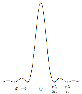
Figure \( 13.5\): The intensity of the diffraction pattern as a function of \(x\).

corresponding to a rather small slit, with a width of only \(100 / \pi \approx 32\) times the wavelength of the wave. We will then use (13.19) to calculate the intensity of the wave at various values of \(z\), in units of \(a\). For small \(z\), the result is shown in Figure \( 13.6\). You can see that the basic beam shape is maintained for a while, as we expected from (13.28). However, wiggles develop immediately. The rather large wiggly diffraction is due to the sharp edges. Below, we will give another example in which the diffraction is much gentler. For intermediate \(z\), shown in Figure \( 13.7\), the wiggles begin to coalesce and dramatically change the overall shape of the beam. At the same time, the beam begins to spread out.

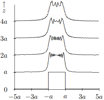
Figure \( 13.6\): The intensity of a wave passing through a slit, for small \(z\).

Finally, in Figure \( 13.8\), we show the approach to the large \(z\) regions, where diffraction takes over completely and the far field diffraction pattern, (13.54), appears.

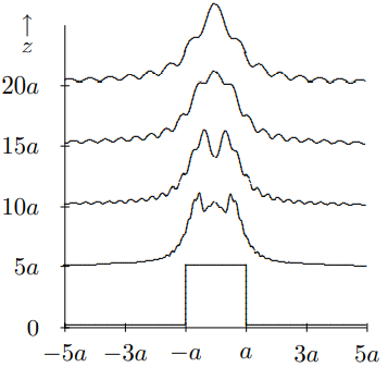
Figure \( 13.7\): The intensity of a wave passing through a slit, for intermediate \(z\).

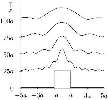
Figure \( 13.8\): The intensity of a wave passing through a slit, as \(z\) gets large.

One more example may be interesting. Suppose that instead of being a simple hole in the opaque screen, the opening is shaded in such a way that the wave disturbance at \(z = 0\) has the form \[f(x, y)=e^{-|x| / a}.\]

The Fourier transform here was done in Chapter 10 in (10.49)-(10.56). Substituting \(\omega \rightarrow k_{x}\) and \(\Gamma \rightarrow 1 / a\) in (10.56) gives \[C\left(k_{x}\right)=\frac{1}{\pi} \frac{a}{1+a^{2} k_{x}^{2}}.\]

This determines the intensity distribution at large \(z\). However, unlike the previous example, this pattern gives very gentle diffraction. For small \(z\), the intensity pattern is shown in Figure \( 13.9\). The sharp point in (13.56) disappears, but otherwise the change is very gradual because the initial pattern is very smooth except at \(x = 0\). For intermediate and large \(z\), the intensity patterns are shown in Figure \( 13.10\) and Figure \( 13.11\).

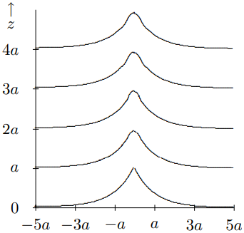
Figure \( 13.9\): The intensity distribution from (13.56) for small \(z\).

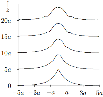
Figure \( 13.10\): The intensity distribution from (13.56) for intermediate \(z\).

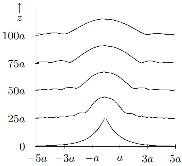
Figure \( 13.11\): The intensity distribution from (13.56) for large \(z\).

Rectangle

Suppose \[f(x, y)-\left\{\begin{array}{l}
1 \text { for }-a_{x} \leq x \leq a_{x} \text { and }-a_{y} \leq y \leq a_{y}, \\
0 \text { otherwise }.
\end{array}\right.\]

This is the product of a single slit pattern in \(x\) with a single slit pattern in \(y\). The Fourier transform is the product of the one-dimensional Fourier transforms \[\begin{aligned}
C\left(k_{x}, k_{y}\right)=& \frac{1}{4 \pi^{2}} \int_{-a_{x}}^{a_{x}} d x e^{-i k_{x} x} \int_{-a_{y}}^{a_{y}} d y e^{-i k_{y} y} \\
&=\frac{\sin \left(k_{x} a_{x}\right)}{\pi k_{x}} \frac{\sin \left(k_{y} a_{y}\right)}{\pi k_{y}}
\end{aligned}\]

Thus the intensity looks approximately like \[I(x, y) \propto \frac{\sin ^{2}\left(2 \pi a_{x} x / r \lambda\right)}{x^{2}} \frac{\sin ^{2}\left(2 \pi a_{y} y / r \lambda\right)}{y^{2}}.\]

Of course, once again, because of the general properties of the Fourier transform, if the rectangle is narrow in \(x\), the diffraction pattern is spread out in \(k_{x}\), and similarly for \(y\).

\(\delta\) “Functions”

As the slit in (13.49) gets narrower, the diffraction pattern spreads out. Of course, the intensity also decreases. The intensity at \(k_{x} = 0\) is related to the Fourier transform of \(f\) at zero, which is just the integral of \(f\) over all \(x\). As the slit gets narrower, this integral decreases. But suppose that we increase the intensity of the incoming beam, as \(a\) decreases, to keep the intensity of the maximum of the diffraction pattern fixed. Ignoring the \(y\) dependence, we require \[f_{a}(x)=\left\{\begin{array}{l}
\frac{1}{2 a} \text { for }-a \leq x \leq a, \\
0 \text { for }|x|>a.
\end{array}\right.\]

The limit of \(f_{a}\) as \(a \rightarrow 0\) doesn’t really exist as a function. It is zero everywhere except \(x = 0\). But it goes to \(\infty\) very fast at \(x = 0\), so that \[\lim _{a \rightarrow 0} \int d x f_{a}(x)=1\]

It is extraordinarily convenient to invent an object with these properties, called a “\(\delta\)-function”. That is, \(\delta(x)\) has the property that it is zero except at \(x = 0\), and that \[\int d x \delta(x)=1.\]

In fact, this object makes a kind of mathematical sense, so long as you do not square it. \(\delta\)-functions can be manipulated like ordinary functions, added together, multiplied by constants or smooth functions — \(\delta\)-functions of different variables can even be multiplied — just don’t square them! For example, a delta function can be multiplied by an ordinary continuous function: \[f(x) \delta(x)=f(0) \delta(x)\]

where the equality follows because the delta function vanishes except at \(x = 0\), so that only the value of \(f\) at 0 matters.

Now it should be clear from (13.63) and (13.64) that the Fourier transform of \(\delta(x)\) is just a constant: \[C(k)=\frac{1}{2 \pi} \int d x e^{-i k x} \delta(x)=\frac{1}{2 \pi}.\]

The diffraction pattern for this thing is thus very boring. There is uniform illumination at all angles.

Of course, in physics, we can’t make \(\delta\)-functions. However, if \(a\), in (13.61) is much smaller than the wavelength of the wave, then it might as well be a \(\delta\)-function, because it only matters what \(C(k_{x})\) is for \(k_{x}<k=2 \pi / \lambda\). Larger \(k_{x}\) correspond to exponential waves that die off rapidly with \(z\). But for such \(k_{x}\), the product \(k_{x}a\) is very small, thus \[C\left(k_{x}\right)=\frac{1}{2 \pi} \frac{\sin k_{\underline{x}} a}{k_{x} a} \rightarrow \frac{1}{2 \pi}\left(1-\frac{\left(k_{\underline{x}} a\right)^{2}}{6}+\cdots\right) \approx \frac{1}{2 \pi}\]

and we still get uniform diffraction over all angles.

Moral: \(\delta\)-functions are simply a convenience. When physicists talk about a \(\delta\)-function, they mean (or at least they should mean) a function like \(f_{a}(x)\), where \(a\) is smaller than any physical distance that is important in the problem. Once \(a\) gets that small, it is often easier to keep track of the math when you go all the way to the unphysical limit, \(a = 0\).

Some Properties of \(\delta\)-Functions

The Fourier transform of a \(\delta\)-function is a complex exponential: \[\text { if } f(x)=\delta(x-a) \text { then } C(k)=\frac{1}{2 \pi} e^{-i k a} \text { . }\]

The Fourier transform of a complex exponential is a \(\delta\)-function: \[\text { if } f(x)=e^{-i \ell x} \text { then } C(k)=\delta(k-\ell).\]

A \(\delta\)-function can be reached as a limit in a variety of different ways. For example, from (13.68), we would expect that as \(a \rightarrow \infty\), the Fourier transform of (13.49) should approach a \(\delta\)-function: \[\lim _{a \rightarrow \infty} \frac{\sin k_{x} a}{k_{x}}=\delta\left(k_{x}\right) \text { . }\]

Dimension from Two

Using \(\delta\)-functions, we can say more elegantly what is meant by the statement we made above that if \(f(x, y)\) does not depend on \(y\), the problem is one-dimensional. If we look at the limit of (13.58) as \(a_{y} \rightarrow \infty\), it goes over into (13.49). In other words, when a rectangle is infinitely long, it is a slit. In this limit, the Fourier transform, (13.59) goes into \[\frac{\sin \left(k_{x} a_{x}\right)}{\pi k_{x}} \delta\left(k_{y}\right).\]

This is the real meaning of (13.50). It is one-dimensional in the sense that \(k_{y}\) is stuck at 0. There is no diffraction in the \(y\) direction.

Many Narrow Slits

An interesting application of δ-functions is to the diffraction pattern for several narrow slits. We will use this later in various ways. Consider a function, \(f(x, y)\) of the form \[\sum_{j=0}^{n-1} \delta(x-j b)\]

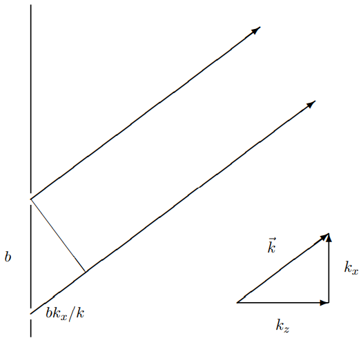
Figure \( 13.12\): If \(b k_{x} / k=n \lambda\), the interference is constructive.

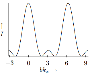
Figure \( 13.13\): The diffraction pattern for three narrow slits.

This describes a series of \(n\) narrow slits⁹ at \(x = 0\), \(x = b\), \(x = 2b\), etc., up to \(x = (n − 1)b\). The Fourier transform of (13.71) is a sum of contributions from the individual \(\delta\)-functions,

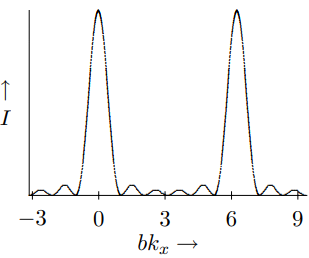
Figure \( 13.14\): The diffraction pattern for 6 narrow slits.

from (13.67) and (13.68) \[C\left(k_{x}, k_{y}\right)=\delta\left(k_{y}\right) \frac{\perp}{2 \pi} \sum_{j=0}^{n-1} e^{-i j b k_{x}}.\]

But the sum is a geometric series that can be done explicitly: \[\begin{gathered}
\sum_{j=0}^{n-1} e^{-i j b k_{x}}=\frac{1-e^{-i n b k_{x}}}{1-e^{-i b k_{x}}} \\
=\frac{e^{-i n b k_{x} / 2}\left(e^{i n b k_{x} / 2}-e^{-i n b k_{x} / 2}\right)}{e^{-i b k_{x} / 2}\left(e^{i b k_{x} / 2}-e^{-i b k_{x} / 2}\right)}=e^{-i(n-1) b k_{x} / 2} \frac{\sin n b k_{x} / 2}{\sin b k_{x} / 2} .
\end{gathered}\]

Thus the diffraction pattern intensity is proportional to \[\frac{\sin ^{2} n b k_{x} / 2}{\sin ^{2} b k_{x} / 2}.\]

For \(n = 2\), (13.74) is just \[4 \cos ^{2} \frac{b k_{x}}{2}=2\left(1+\cos b k_{x}\right).\]

This is the problem with which we started the chapter. When \(b k_{x}=2 m \pi\) for integer \(m\), then the wave from one slit travels farther than the wave from the other by \(m \lambda\), where \(\lambda=2 \pi / k\) is the wavelength. Thus for \(b k_{x}=2 m \pi\) the interference is constructive, as illustrated in figure 13.12.

For larger \(n\), we still get constructive interference for \(b k_{x}=2 m \pi\), but the maxima are sharper, because with more slits, there are more possibilities for destructive interference at other angles. In Figure \( 13.13\) and Figure \( 13.14\), we plot (13.74) versus \(bk_{x}\) from (−\(\pi\) to \(3\pi\) so that you can see two full periods) for \(n = 3\) and \(6\). Notice the appearance of \(n − 2\) secondary maxima between the primary maxima of the intensity. We will return to these relations when we discuss diffraction gratings.

____________________________________

⁶Again, this is simplistic, ignoring complications from the boundaries in the same way as (13.15).
⁷Note that \(\sin k a / k\) is well-defined (\(= a\)) at \(k = 0\).
⁸Here we are assuming small angles, so that \(\sin \theta \approx \tan \theta\). In our discussion of diffraction gratings below, we will see what happens when the difference in important.
⁹“Narrow” here means narrow compared to the wavelength of the light — see the moral above.