13.3: Small and Large z

But what do we do with it? The integral in (13.19) is too complicated to do analytically. Below, we will give some examples of how it works by doing the integral numerically. However, for small \(z\) and for large \(z\), the integral simplifies in different ways.

Small \(z\)

For sufficiently small \(z\), we would expect on physical grounds that we really have produced a beam and projected an image of the function, \(f(x, y)\). To see this explicitly, we will use the fact that for a particular (well behaved) \(f(x, y)\), the Fourier transform \(C(k_{x}, k_{y})\) is a function that goes to zero for \[k \equiv \sqrt{k_{x}^{2}+k_{y}^{2}} \gg 1 / L\]

for some \(L\) much larger than the wavelength. The distance \(L\) is determined by the smoothness of \(f(x, y)\). Typically, \(L\) is the size of the smallest important feature in \(f(x, y)\), the smallest distance over which \(f(x, y)\) changes appreciably. We saw this in our discussion of Fourier transforms in connection with signals in Chapter 10. We will see more examples below. We can expand \(k_{z}z\) in the exponential in a Taylor expansion, \[\begin{aligned}
&k_{z} z=z \sqrt{\omega^{2} / v^{2}-k_{x}^{2}-k_{y}^{2}} \\
&=\frac{z \omega}{v} \sqrt{1-\frac{v^{2}\left(k_{x}^{2}+k_{y}^{2}\right)}{\omega^{2}}} \\
&\approx \frac{z \omega}{v}-\frac{z v\left(k_{x}^{2}+k_{y}^{2}\right)}{2 \omega}
\end{aligned}\]

Because of (13.25), the largest value of \(\sqrt{k_{x}^{2}+k_{y}^{2}}\) that we need in the integral, (13.19) \[\psi(\vec{r}, t)=\int d k_{x} d k_{y} C\left(k_{x}, k_{y}\right) e^{i \vec{k} \cdot \vec{r}-i \omega t} \text { for } z>0\]

is of order \(1/L\). For much larger values, the integrand is zero. Thus the largest possible value of the second term in the expansion (13.26) that matters in the integral, (13.19) is of the order of \[\frac{z v}{2 \omega L^{2}}.\]

Therefore, if \(L\) is finite and \(z\) is small \(\left(\ll \omega L^{2} / v\right)\), the second term is small and we can keep only the first term, \(z \omega / v\). Then putting this back into the integral, (13.19), we have \[\begin{gathered}
\psi(\vec{r}, t)=\int d k_{x} d k_{y} C\left(k_{x}, k_{y}\right) e^{i \vec{k} \cdot \vec{r}-i \omega t} \\
\approx \int d k_{x} d k_{y} C\left(k_{x}, k_{y}\right) e^{i\left(k_{x} x+k_{y} y+z \omega / v-\omega t\right)} \\
\approx \int d k_{x} d k_{y} C\left(k_{x}, k_{y}\right) e^{i\left(k_{x} x+k_{y} y\right)} e^{i(z \omega / v-\omega t)} \approx f(x, y) e^{i \omega(z-v t) / v}
\end{gathered}\]

This is just what we expect — a beam with the shape of the original function, propagating in the \(z\) direction with velocity \(v\).

The result (13.28) begins to break down when the next term in the Taylor series, (13.26), becomes important. That is when \[\frac{z v\left(k_{x}^{2}+k_{y}^{2}\right)}{\omega} \approx 1\]

Thus \[z \approx \frac{\omega L^{2}}{v}=\frac{2 \pi L^{2}}{\lambda}\]

marks the transition from a simple beam to the onset of important diffraction effects.

If \(L = 0\), which is the situtation in the example of a single slit of width \(2a\), that we will analyze in detail later, important diffraction effects start immediately because the slit has sharp edges. However, the beam maintains some semblance of its original size until \(z \approx a^{2} / \lambda\).

For z larger than \(\omega L^{2} / v\), the \(k_{x}\) and \(k_{y}\) dependence from the \(e^{i k_{z} z}\) factor cannot be ignored. In general, the evaluation of the integral, (13.19), is very hard. However, for very large \(z, z \gg L\), we can use a physical argument to find the result of the integral, (13.19).

Large \(z\)

Suppose that you are very far away, at a point \(\vec{R}=(X, Y, Z)\), \[(x, y, z)=(X, Y, Z) \text { for } Z \gg \omega L^{2} / v.\]

Then you cannot see the details of the shape of the opening or other details of \(f(x, y)\), only its position. The wave you detect at some far-away point must have come from the opening and if you are far enough away, it is almost a plane wave. This is called “Fraunhofer” or “far-field” diffraction. If this condition is not satisfied, the problem is called “Fresnel” or “near-field” diffraction. For the light to actually reach your eye in the far-field situation, the propagation vector must point from the opening to you. The situation is depicted in the diagram in Figure \( 13.3\). In the near-field region, the spreading due to diffraction is of the same order as the size of the opening. For much larger \(Z\), in the far-field region, the \(\vec{k}\) vector must point back to the opening.

Thus the only contribution to the integral, (13.19), \[\psi(\vec{r}, t)=\int d k_{x} d k_{y} C\left(k_{x}, k_{y}\right) e^{i \vec{k} \cdot \vec{r}-i \omega t} \text { for } z>0\]

that counts is that proportional to \(e^{i \vec{k} \cdot \vec{R}}\) where \(\vec{k}\) points from the opening to your eye. Because the integrand in (13.19) has a factor of \(C(k_{x}, k_{y})\), the amplitude of the wave is proportional to \(C(k_{x}, k_{y})\) where \[\left(k_{x}, k_{y}, k_{z}\right)=\left(k_{x}, k_{y}, \sqrt{\omega^{2} / v^{2}-k^{2}}\right) \propto(X, Y, Z).\]

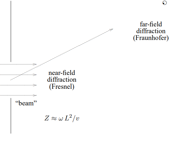
Figure \( 13.3\): The basic diffraction problem — making a beam.

The amplitude is also inversely proportional to \[R=\sqrt{X^{2}+Y^{2}+Z^{2}},\]

because the intensity must fall off as \(R^{−2}\), as in a spherical wave, by energy conservation.

There are other factors that contribute to the variation of the amplitude besides \(C(k_{x}, k_{y})\) (we will see one below). However, typically, all the other factors are very slowly varying and can be ignored. Thus we expect that the intensity for large \(Z\) is approximately \[\frac{\left|C\left(k_{x}, k_{y}\right)\right|^{2}}{R^{2}},\]

where \(\vec{k}\) and \(\vec{R}\) are related by (13.32). \[\left(k_{x}, k_{y}, k_{z}\right)=\left(k_{x}, k_{y}, \sqrt{\omega^{2} / v^{2}-k^{2}}\right) \propto(X, Y, Z)\]

which implies \[\frac{k_{x}}{X}=\frac{k_{y}}{Y}=\frac{k_{z}}{Z}=\frac{k}{R}=\frac{\omega / v}{R},\]

or \[k_{x}=\frac{k X}{R}, \quad k_{y}=\frac{k Y}{R}.\]

Now here is the point! Inserting (13.36) into (13.24) \[C\left(k_{x}, k_{y}\right)=\frac{1}{4 \pi^{2}} \int d x d y f(x, y) e^{-i\left(k_{x} x+k_{y} y\right)}\]

gives the integral in (13.14) that came from our physical argument about interference! \[\int d x \int d y f(x, y) e^{i k(R+\Delta \ell)}=e^{i k R} \int d x \int d y f(x, y) e^{-i(x X+y Y) k / R}\]

Thus our description of the wave for \(z > 0\) as a forced oscillation problem contains the same factor that describes the interference of all the paths that the wave can take from the opening to \(\vec{R}\). The advantage of our present approach is that it is a real derivation.

We can also write this result in terms of angles: \[\sin \theta_{x}=\frac{X}{R}=\frac{k_{x} v}{\omega}, \sin \theta_{y}=\frac{Y}{R}=\frac{k_{y} v}{\omega}\]

where \(\theta_{x}\) and \(\theta_{y}\) are the angles of the vector \(\vec{r}\) from the \(X = y = 0\) line in the \(x\) and \(y\) directions. Or equivalently, \[X=\frac{Z k_{x}}{\sqrt{\omega^{2} / v^{2}-k_{x}^{2}-k_{y}^{2}}}, \quad y=\frac{Z k_{y}}{\sqrt{\omega^{2} / v^{2}-k_{x}^{2}-k_{y}^{2}}}\]

This is illustrated in the diagram in Figure \( 13.4\).

Stationary Phase

Mathematically, (13.32) \[\left(k_{x}, k_{y}, k_{z}\right)=\left(k_{x}, k_{y}, \sqrt{\omega^{2} / v^{2}-k^{2}}\right) \propto(X, Y, Z)\]

arises for large \(Z\) becasue the phase of the exponential in (13.19) \[\psi(\vec{r}, t)=\int d k_{x} d k_{y} C\left(k_{x}, k_{y}\right) e^{i \vec{k} \cdot \vec{r}-i \omega t} \text { for } z>0\]

is very rapidly varying as a function of \(k_{x}\) and \(k_{y}\) except for special values of \(k_{x}\) and \(k_{y}\) where the derivatives of the phase with respect to \(k_{x}\) and \(k_{y}\) vanish. If the function is centered at \(x = y = 0\) and is smooth,⁵ the \(k\) derivatives of \(C(k_{x}, k_{y})\) are of order \(L\) and are

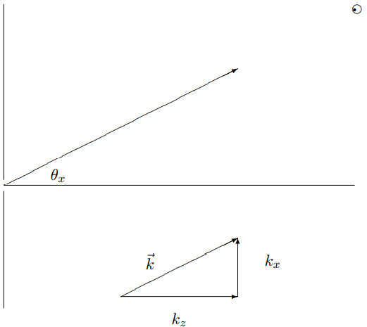
Figure \( 13.4\):

irrelevant. Thus the contribution comes from \(k_{x}\), \(k_{y}\) such that \[\begin{aligned}
\frac{\partial}{\partial k_{x}}\left(X k_{x}+Y k_{y}+Z \sqrt{\omega^{2} / v^{2}-k_{x}^{2}-k_{y}^{2}}\right) &=X-\frac{Z k_{x}}{\sqrt{\omega^{2} / v^{2}-k_{x}^{2}-k_{y}^{2}}}=0, \\
\frac{\partial}{\partial k_{y}}\left(X k_{x}+Y k_{y}+Z \sqrt{\omega^{2} / v^{2}-k_{x}^{2}-k_{y}^{2}}\right) &=Y-\frac{Z k_{y}}{\sqrt{\omega^{2} / v^{2}-k_{x}^{2}-k_{y}^{2}}}=0,
\end{aligned}\]

which is equivalent to (13.38). A careful evaluation of the integral, taking account of the \(k_{x}\) and \(k_{y}\) dependence in the neighborhood of the critical value determined by (13.38) yields an additional factor in the amplitude of the wave of \[\frac{Z}{r^{2}}=\frac{\cos \theta}{r}\]

where \(\theta\) is the angle of the vector \(\vec{r}\) to the \(z\) axis. We expected the \(/r\) factor because of the spreading of the diffracted wave with distance. The factor of \(\cos \theta\) is actually the only place where the details of the boundary condition at infinity, (13.21), enter into our expression for the diffracted wave. This factor guarantees that the diffracted wave vanishes as we go to the surface of the opaque screen far from the opening. This is analogous to the “obliquity” factor \((1+\cos \theta) / 2\), in the Fresnel-Kirchhoff diffraction theory. The difference between the two is due to the different boundary conditions (our infinite flat barrier versus the lack of incoming spherical waves). We will usually ignore this factor, and indeed it generally does not make much difference where diffraction is important in the forward direction. The important thing is that everything else about the diffraction in the far-field region is determined just by linearity, translation invariance and local interactions.

Spot Size

A useful way to think about the transition from near-field (Fresnel) to far-field (Fraunhofer) diffraction is to consider the size of the spot formed by the beam of Figure \( 13.3\) as a function of \(z\). This is a competition between two effects. Increasing the size of the opening makes the spot size larger at small \(z\). However, decreasing the size of the opening increases the spread in \(k_{x}\), thus increasing the diffraction, and making the spot size larger at large \(z\). For a given \(z\), the best you can do is to choose the size of your opening so that these two effects are of the same order of magnitude. Suppose that the size of your opening is \(\ell\). Then the spread in \(k_{x}\) is of order \(2 \pi / \ell\). At large \(z\), the beam spreads into a cone with an opening angle of order \[\theta \approx \frac{\lambda}{\ell}.\]

Thus when \[\frac{\lambda}{\ell} \approx \frac{\ell}{z},\]

the spreading of the spot due to diffraction is of the same order of magnitude as the size of the opening. We conclude that to minimize the spot size for a given \(z\), you should choose an opening of size \[\ell \approx \sqrt{\lambda z}.\]

The relation, (13.41), up to factors of \(\pi\), is what defines the region of Fresnel diffraction in Figure \( 13.3\). Another way of summarizing the result of this discussion is that for \[z \gg \frac{\ell^{2}}{\lambda},\]

the spreading due to diffraction is much larger than the spreading due to the size of the opening. This defines the region of far-field, or Fraunhofer diffraction.

Angles

What happens if the plane wave in (13.15) is coming in toward the opaque barrier at an angle, rather than head on? To be specific, suppose that the \(\vec{k}\) vector of the wave makes an angle \(\theta\) with the perpendicular in the \(x\)-\(z\) plane, so that \[k_{z}=k \cos \theta, \quad k_{x}=k \sin \theta.\]

Then it is reasonable to assume that the analog of (13.15), the amplitude of the wave in the \(z = 0\) plane, is⁶ \[f_{\theta}(x, y)=f(x, y) e^{i x k \sin \theta}\]

where the additional \(x\) dependence has simply been inherited from the \(x\) dependence of the incoming wave. We can write the Fourier transform of \(f_{\theta}\) in terms of that of \(f\) as follows: \[\begin{aligned}
&f_{\theta}(x, y)=\int d k_{x} d k_{y} C\left(k_{x}, k_{y}\right) e^{i\left(k_{x} x+k_{y} y\right)} e^{i x k \sin \theta} \\
&=\int d k_{x} d k_{y} C\left(k_{x}-k \sin \theta, k_{y}\right) e^{i\left(k_{x} x+k_{y} y\right)}
\end{aligned},\]

which implies \[Cθ(kx, ky) = C(kx − k sin θ, ky).\]

This is entirely reasonable. If the maximum of \(C(k_{x}, k_{y})\) occurs at \(k_{x} \approx 0\), the maximum of \(C_{\theta}(k_{x}, k_{y})\) occurs at \(k_{x}=k \sin \theta\). Thus the diffraction pattern appears where a line through the opening in the direction of the incoming plane wave crosses the screen, just as we would expect from a skew beam.

__________________________

⁵See, however, the discussion on page 383.