13.5: Convolution

There is a rather simple theorem, know as the convolution theorem, that is extremely useful in dealing with Fourier transforms. Suppose that we have two functions, \(f_{1}(x)\) and \(f_{2}(x)\). Define the function \(f_{1} \circ f_{2}\) as follows: \[f_{1} \circ f_{2}(x)=\int_{-\infty}^{\infty} d y f_{1}(x-y) f_{2}(y)\]

This integral will be well defined if \(f_{1}(x)\) and \(f_{2}(x)\) fall off fast enough at infinity (and certainly if they are nonzero only in a finite region of \(x\)). Note that \(f_{1} \circ f_{2}\) is a function of a single variable. It is also symmetric under the exchange of the two functions, because by a simple change of variables \((y \rightarrow x-y)\) \[f_{1} \circ f_{2}(x)=\int_{-\infty}^{\infty} d y f_{1}(x-y) f_{2}(y)=\int_{-\infty}^{\infty} d y f_{1}(y) f_{2}(x-y)=f_{2} \circ f_{1}(x)\]

Now the theorem is that the Fourier transform of the convolution is \(2\pi\) times the product of the Fourier transforms of the two functions. The proof is immediate (all integrals run from −\(\infty\) to \(\infty\)): \[\begin{aligned}
C_{f_{1} \circ f_{2}}(k)=\frac{1}{2 \pi} \int d x e^{i k x} f_{1} \circ f_{2}(x) \\
=& \frac{1}{2 \pi} \int d x e^{i k x} \int d y f_{1}(x-y) f_{2}(y)
\end{aligned}\]

Now we substitute \(x \rightarrow y+z\) and write the integral over \(y\) and \(z\), \[\begin{gathered}
=\frac{1}{2 \pi} \int d z e^{i k(y+z)} \int d y f_{1}(x-y) f_{2}(y) \\
=\frac{1}{2 \pi} \int d z e^{i k z} f_{1}(z) \int d y e^{i k y} f_{2}(y)=2 \pi C_{f_{1}}(k) C_{f_{2}}(k) .
\end{gathered}\]

The two-dimensional analog of (13.79) is a straightforward extension. The two-dimensional convolution is \[f_{1} \circ f_{2}(x, y)=\int d x^{\prime} d y^{\prime} f_{1}\left(x-x^{\prime}, y-y^{\prime}\right) f_{2}\left(x^{\prime}, y^{\prime}\right)\]

\[C_{f_{1} \circ f_{2}}\left(k_{x}, k_{y}\right)=4 \pi^{2} C_{f_{1}}\left(k_{x}, k_{y}\right) C_{f_{2}}\left(k_{x}, k_{y}\right)\]

Repeated Patterns

The convolution theorem can be used to understand many interesting situations. Consider the following very instructive pattern of two wide slits: \[f(x, y)=\left\{\begin{array}{l}
1 \text { for }-a \leq x \leq a \\
1 \text { for }-a \leq x-b \leq a \\
0 \text { otherwise }
\end{array}\right.\]

for \(b > 2a\). A piece of the pattern is shown in Figure \( 13.15\) for \(b = 3.5a\).

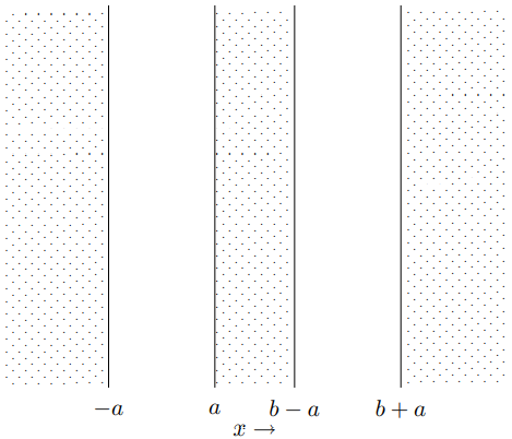
Figure \( 13.15\): A piece of the opaque barrier with two wide slits.

This can be regarded as the convolution of two functions: \[f=f_{1} \circ f_{2}\]

where \[f_{1}(x, y)=\left\{\begin{array}{l}
1 \text { for }-a \leq x \leq a \\
0 \text { otherwise }
\end{array}\right.\]

and \[f_{2}(x, y)=\delta(x) \delta(y)+\delta(x-b) \delta(y)\]

f2(x, y) = δ(x) δ(y) + δ(x − b) δ(y). The corresponding Fourier transforms are, from (13.70) (13.84) (13.85) Cf1 (kx, ky) = sin(kxa) π kx δ(ky) (13.86) and from (13.73) Cf2 (kx, ky) = 1 4π2 cos bkx 2 e−ibkx/2 . Now applying the convolution theorem gives (13.87) Cf1◦f2 (kx, ky) = cos bkx 2 e−ibkx/2 sin(kxax) π kx δ(ky). (13.88) 13.6. PERIODIC f(x, y) 395 Because b > 2a, this describes a pattern that oscillates rapidly on the scale set by 1/b, with an amplitude that varies with the single slit diffraction pattern characterized by size 1/a. The intensity pattern on a distant screen is shown in figure 13.16, for b = 3.5a The dotted line is the pattern for a single wide slit (compare (13.5)).

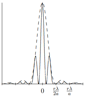
Figure \( 13.16\): The diffraction pattern for two wide slits.