13.6: Periodic f(x, y)

Suppose \(f(x, y)\) is periodic in \(x\) with period \(a\). That is \[f(x+a, y)=f(x, y).\]

Then \(C(k_{x}, k_{y})\) can only be nonzero if

\[k_{x}=\frac{2 \pi n}{a}. \label{13.90}\]

To see this, insert (13.89) into (13.24),

\[C\left(k_{x}, k_{y}\right)=\frac{1}{4 \pi^{2}} \int d x d y\, f(x+a, y) e^{i\left(k_{x} x+k_{y} y\right)}. \label{13.91}\]

If we change variables from \(x \rightarrow x-a\), Equation \ref{13.91} is

\[\begin{align} C\left(k_{x}, k_{y}\right) &= \frac{1}{4 \pi^{2}} \int d x d y \,f(x, y) e^{i\left(k_{x} x-k_{x} a+k_{y} y\right)} \\[4pt] &= e^{-i k_{x} a} C\left(k_{x}, k_{y}\right) \label{13.92} \end{align}\]

because the constant phase factor can be taken outside the integral. Equation \ref{13.90} follows because Equation \ref{13.92} implies that either \(C\left(k_{x}, k_{y}\right)=0\) or \(e^{-i k_{x} a}=1\).

An example of this general principle is Equation \ref{13.74}. In the limit that \(n \rightarrow \infty\), (13.74) goes to 0 except for \(k_{x}=2 \pi m / b\) for integer \(m\) (where it is infinite). This example is simple because the slits are narrow, so the intensity is independent of \(m\). However, with repeated wide slits, or some more complicated pattern, we could use the convolution theorem and (13.74) to see that (13.90) emerges as \(n \rightarrow \infty\). The details of the pattern of each slit will then determine the relative intensity of the diffraction pattern at different \(m\).

Thus any infinite regular pattern produces a discrete sequence of \(k\)’s. For example, a transmission diffraction grating, that consists of lots of equally spaced lines in the \(y\) direction with \(x\) separation \(a\) on a transparent substrate, produces a \(C(k_{x}, k_{y})\) that is nonzero only for \(k_{y} = 0\) (because there is no \(y\) dependence at all) and \(k_{x}=2 n \pi / a\). Then (13.19) becomes \[\sum_{n} C_{n} e^{i\left(2 n \pi x / a+z \sqrt{\omega^{2} / v^{2}-(2 n \pi / a)^{2}}-\omega t\right)}\]

This describes a linear superposition of plane waves fanning out at angles in the \(x\) direction given by

\[\sin \theta_{n}=\frac{2 \pi n v}{a \omega}=\frac{n \lambda}{a}\]

as shown in Figure \( 13.17\).

Typically, for a transmission grating, most of the light goes into the central line, which is to say that you can see right through the grating. Note that the even spacing in \(\sin \theta_{n}\) in (13.94) corresponds to an increasing spacing of the lines projected onto a screen at fixed large \(z\) (for example, a screen like your retina!) because the distance along the screen is determined by \[\tan \theta_{n}=\frac{n \lambda}{\sqrt{a^{2}-n^{2} \lambda^{2}}}.\]

There is a maximum value of \(n\), above which no propagating wave is produced (because it corresponds to \(\sin \theta>1\) and thus imaginary \(k_{z}\)).

Note also the dependence of (13.94) on wavelength. The larger the wavelength of the light, the larger the angles in the pattern from the diffraction grating. This, of course, is why the diffraction grating is useful. It can separate light of different frequencies. The different colors of the rainbow are spread out along a line, for each value of \(n\). This is illustrated in the Figure \( 13.18\), for three frequencies, blue light with wavelength 4300 \(\AA\), green light with wavelength 5200 \(\AA\) and red light with wavelength 6300 \(\AA\), incident on a diffraction grating with 10,000 lines per inch. We have shown (13.95) for \(n\) = −3 to 3 and labeled the colors for the \(n = 1\) secondary maximum. As you see, in a realistic grating, the angles of diffraction can be large, and it is a very bad idea to use a small angle approximation.

13.6.1 Twisting the Grating

Some interesting examples of the effects discussed in (13.48) occur when the incoming light wave comes at the grating at an angle with respect to the perpendicular. Starting with the

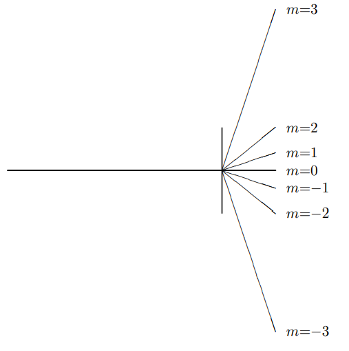
Figure \( 13.17\): A transmission diffraction grating splits a beam of a single frequency.

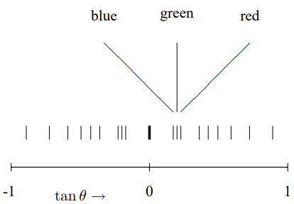
Figure \( 13.18\): The pattern of three frequencies of light from a grating.

grating lines in the \(y\) direction and the grating in the \(x\)-\(y\) plane, there are two different effects.

Twisting Around the \(y\) Axis

Suppose that the light comes in at an angle \(\theta_{in}\) from the perpendicular in the \(x\)-\(z\) plane. Then from (13.48), \[C_{\theta_{\mathrm{in}}}\left(k_{x}, k_{y}\right)=C\left(k_{x}-k \sin \theta_{\mathrm{in}}, k_{y}\right)\]

where \(C\) is Fourier transform for the perpendicular grating, \[C\left(k_{x}, k_{y}\right) \neq 0 \quad \text { for } \quad k_{y}=0, k_{x}=\frac{2 \pi n}{a}.\]

Thus \[\begin{gathered}
C_{\theta_{\text {in }}}\left(k_{x}, k_{y}\right) \neq 0 \quad \text { for } \\
k_{y}=0, k_{x}=k \sin \theta_{\text {in }}+\frac{2 \pi n}{a}
\end{gathered}\]

or \[\sin \theta=\frac{k_{x}}{k}=\sin \theta_{\mathrm{in}}+\frac{n \lambda}{a}.\]

In other words, \(\sin \theta\) is simply displaced by \(\sin \theta_{\mathrm{in}}\). For example, this means that if \(\theta=\pi / a\), the pattern is exactly the same, but the central maximum has moved over, as shown in Figure \( 13.19\).

Twisting Around the \(x\) Axis

Suppose that the light comes in at an angle \(\theta\) from the perpendicular in the \(y\)-\(z\) plane. Then from (13.48). \[C_{\theta_{\text {in }}}\left(k_{x}, k_{y}\right)=C\left(k_{x}, k_{y}-k \sin \theta_{\text {in }}\right) .\]

Now instead of being 0, \(k_{y}\) is fixed at \(k \sin \theta_{\text {in }}\) \[k_{y}=k \sin \theta_{\text {in }}, \quad k_{x}=\frac{2 \pi n}{a} \text { . }\]

Now the diffracted waves make nontrivial angles from the perpendicular both in \(x\) and in \(y\) \[\sin \theta_{y}=\frac{k_{y}}{\sqrt{k_{y}^{2}+k_{z}^{2}}}=\frac{k_{y}}{\sqrt{k^{2}-k_{x}^{2}}}=\frac{\sin \theta_{\mathrm{in}}}{\sqrt{1-n^{2} \lambda^{2} / a^{2}}}

and \[\sin \theta_{x}=\frac{k_{x}}{\sqrt{k_{x}^{2}+k_{z}^{2}}}=\frac{k_{x}}{\sqrt{k^{2}-k_{y}^{2}}}=\frac{n \lambda}{a \cos \theta_{\mathrm{in}}}.\]

Again, as in (13.95), what we see if we project the pattern onto a perpendicular screen at fixed \(z\) are the tangents, \[(x, y)_{\text {screen }}=z\left(\tan \theta_{x}, \tan \theta_{y}\right),\]

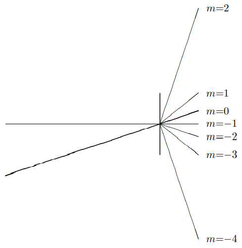
Figure 13.19: The pattern for a beam at an angle, \(\theta_{\text {in }}=\arcsin \lambda / a\).

where \[\tan \theta_{x}=\frac{k_{x}}{k_{z}}, \quad \tan \theta_{y}=\frac{k_{y}}{k_{z}} .\]

Thus the diffraction pattern appears curved. What one sees on a screen or a retina is the colors of the rainbow spread out along a curved line. This is shown in Figure \( 13.20\), where we plot \(\tan \theta_{x}\) versus \(\tan \theta_{y}\) for a light source and grating as in (13.18), above, but with \(\sin \theta_{\text {in }}=0.5\). Note that the pattern has not only curved, it has spread out, compared to (13.18). Here you really see the three-dimensional \(\vec{k}\) vector in action. As \(\tan \theta_{y}\) increases, for fixed \(k_{x}\), \(\tan \theta_{x}\) increases as well, because \(k_{z}\) decreases.

Resolving Power

The discussion so far has assumed that the diffraction grating is truely periodic. But this is only possible if the grating is infinite! In a finite grating, only the middle is periodic. The edges break the periodicity. In a grating consisting of only a finite number of grooves, \(n\), the diffraction peaks are not infinitely sharp. They are not delta functions. However, as discussed at the beginning of this section, we actually already know what they look like in the finite

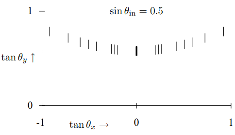
Figure \( 13.20\): The diffraction pattern from a twisted grating.

case because we have solved the problem of diffraction from \(n\) evenly spaced narrow slits, in (13.74). In the general situation for \(n\) identical grooves, the intensity looks like (13.74) multiplied by some slowly varying function that depends on the shape of the grooves (by the convolution theorem, (13.79)). The important consequence of this is that the shape of a diffraction peak for an \(n\)-slit grating is roughly given by (13.74).

The shape of the diffraction peak is important for the following practical question. Suppose that you have a beam of light that consists of a superposition of light of two different frequencies. How close together do the frequencies have to be before their nontrivial diffraction peaks melt together, so that you cannot use your diffraction grating to distinguish them? The larger the number of grooves in the grating, the sharper the diffraction peaks and the easier it is to distinguish different frequencies.

Rayleigh’s criterion is an historically important way of answering this question. Rayleigh assumed that it would be possible to distinguish the diffraction maxima from equally intense waves of slightly different wavelengths if the maximum of one frequency coincides with the first minimum of the other. For a grating of 6 lines, this criterion is illustrated in Figure \( 13.21\). The solid line is the total intensity of a wave consisting of two slightly different frequencies. The contributions from the separate frequency components are indicated by the dotted and dashed lines.

Any such fixed criterion for resolving power should be regarded not as a fact about nature, but as a conventional definition that facilitates communication between experimenters. It is always possible to do better than any given definition by accumulating accurate data on the line shape and modeling the details.

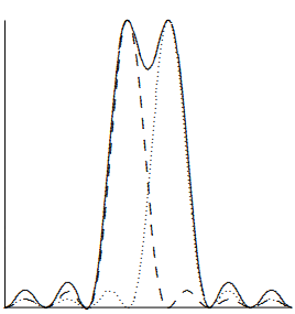
Figure \( 13.21\): Rayleigh’s criterion for a grating with 6 lines.

Blazed Gratings

As a spectroscope, the transmission diffraction grating has a disadvantage compared to a prism. The difficulty is that, as we noted above, most of the light impinging on the grating goes right through and is not split into its component frequencies. This is a very serious problem in devices in which the total amount of light is limited. It is often important to have the bulk of the light going into a single nonzero value of \(n\) in (13.94). Then nearly all of the photons can be used for the measurement, rather than being wasted in the \(n = 0\) maximum (which carries no information about the frequency). As we argued above, there is no theoretical reason why such a thing cannot be done. The general principles of translation invariance and local interactions determine the possible angles of diffraction, but not how much light goes to which angle.

In fact, there is a practical and widely used method in reflection gratings. A reflecting surface with a series of evenly spaced parallel lines scored into it acts as a reflection grating, as illustrated in Figure \( 13.22\). This shows a reflection grating in which the predominant reflection of a beam coming in perpendicular to the plane of the grating is also perpendicular. What we want instead is shown in Figure \( 13.23\). To construct such a grating, you can shape the grooves in the grating so that the specular reflection from the individual grooves directs the beam into the nontrivial diffraction maximum, as shown in Figure \( 13.24\).

To do this, you can choose the angle of the blaze to be half the angle of the first maximum, \(\theta_{1}=2 \pi v / a \omega\), in (13.94), as shown in the blow-up of a groove in figure 13.25.

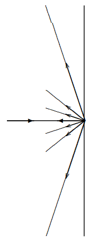
Figure \( 13.22\): A reflection diffraction grating splits a beam of a single frequency.

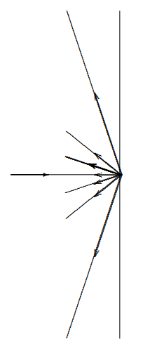
Figure \( 13.23\): A blazed grating directs the beam into a nontrivial diffraction maximum.

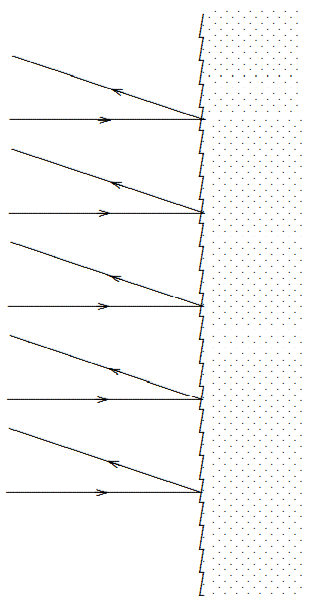
Figure \( 13.24\): The grooves of a blazed grating.

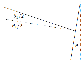
Figure \( 13.25\): \(\theta \approx \theta_{1} / 2.\)