13.9: Fringes and Zone Plates

Holographic Image of a Point

One of the simplest of holographic images is the image of a single point. If a plane wave encounters a very small object in its path, the object will produce a spherical wave. If the plane wave and the spherical wave then are absorbed by a photographic plate, as shown in Figure \( 13.34\), an interference pattern is produced in the form of concentric circles, or fringes.

Specifically, suppose that the plane wave is propagating in the \(z\) direction, the photographic plate is in the \(x\)-\(y\) plane at \(z = z_{0}\) and we put the origin of our coordinate system at the position of the source of the spherical wave, as shown in Figure \( 13.34\). Then the linear combination of plane wave plus spherical wave has the form (ignoring polarization) \[A e^{i k z}+\frac{B}{r} e^{i k r},\]

where \(r=\sqrt{x^{2}+y^{2}+z^{2}}\). We will assume, for simplicity, that \(A\) and \(B\) are real which means that the two waves are in phase at the object. The intensity of the wave at \(z = z_{0}\), on the photographic plate is therefore \[A^{2}+\frac{B^{2}}{r_{0}^{2}}+\frac{2 A B}{r_{0}} \cos \left[k\left(r_{0}-z_{0}\right)\right]\]

where \(r_{0}\) is the distance from the object for a point in the \(z = z_{0}\) plane, \[r_{0}=\sqrt{z_{0}^{2}+R^{2}}\]

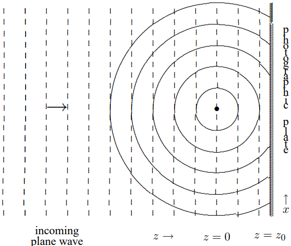
Figure \( 13.34\): Fringes.

and \[R=\sqrt{x^{2}+y^{2}}\]

is the distance from the \(z\) axis in the \(x\)-\(y\) plane. The intensity depends only on \(R\), as it must because of the symmetry of the system under rotations around the \(z\) axis.

Usually, we are interested in the region, \(z_{0} \gg R\), because, as we will see, the intensity pattern is most interesting for small \(R\). In this region, the distance, \(r_{0}\) is very nearly equal to \(z_{0}\). We can ignore the variation of \(r_{0}\) in the amplitude, \(B / r_{0}\). However, there is interesting dependence in the cosine term in (13.133). In this term, we can expand \(r_{0}\) in a Taylor series around \(R=z_{0}\), \[r_{0}=z_{0} \sqrt{1+R^{2} / z_{0}^{2}}=z_{0}+\frac{1}{2} \frac{R^{2}}{z_{0}}+\cdots\]

Putting all this together, the intensity is given approximately for \(z_{0} \gg R\) by \[A^{2}+\frac{B^{2}}{z_{0}^{2}}+\frac{2 A B}{z_{0}} \cos \frac{k R^{2}}{2 z_{0}}.\]

The intensity pattern, (13.137), describes concentric circular “zones” of intensity variation. The zones can be labeled by the maxima and minima of the cosine, at \[\frac{k R^{2}}{2 z_{0}}=n \pi\]

or \[R^{2}=n \lambda z_{0}\]

where \(\lambda\) is the wavelength of the wave. For \(n\) even, the cosine has a maximum and for \(n\) odd, a minimum. The intensity variation is greatest if the plane wave and the spherical wave have approximately the same amplitude at the plate, \[\frac{B}{z_{0}}=A\]

Then the amplitude actually goes to zero at the minima. The intensity distribution as a function of \(R\) is shown in Figure \( 13.35\). The positions of the maxima and minima, or “zones,” are shown on the \(R\) axis. On the photographic plate, this intensity distribution gives rise to circular fringes.

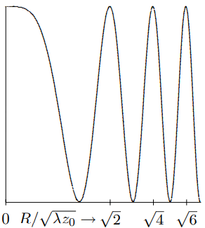
Figure \( 13.35\): The intensity distribution.

If the plate is developed and illuminated by a plane wave, the original spherical wave is reproduced along with another spherical wave moving inward toward a point on the \(z\) axis a distance \(z_{0}\) beyond the plate, as shown in Figure \( 13.36\). This wave is the real image of Figure \( 13.33\). When a plane wave (dotted lines) illuminates the photographic plate produced in Figure \( 13.34\), diverging (dotted lines) and converging (solid lines) spherical waves are produced.

Zone Plates

The hologram of Figure \( 13.34\) can be used to bring part of plane wave to a focus. The converging spherical wave shown in Figure \( 13.36\) is much stronger than the rest of the wave disturbance at the focus, \(z=2 z_{0}\), \(x=y=0\), because the amplitude of this part of the wave

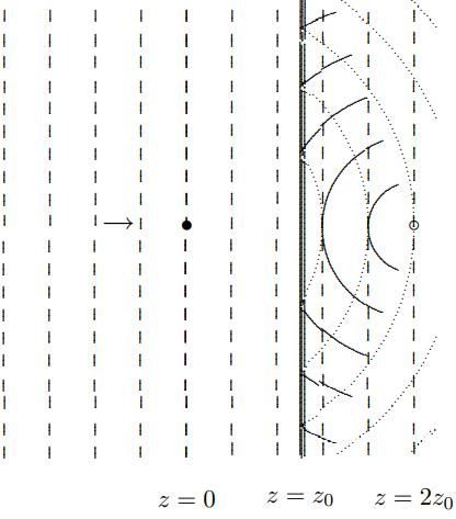
Figure \( 13.36\): A plane wave illuminating the photographic plate.

increases as it approaches the focus. It has the form \[\frac{1}{r^{\prime}} e^{i k r^{\prime}}\]

where \[r^{\prime}=\sqrt{\left(z-2 z_{0}\right)^{2}+x^{2}+y^{2}}.\]

The same effect can be produced with a cartoon version of the photographic plate made by taking a transparent plate and blacking out the zones for negative \(n\) in (13.138) where the intensity distribution is less than half the maximum. For example, the first negative zone is the region \(\lambda z_{0} / 2<R^{2}<3 \lambda z_{0} / 2\). The second is the region \(5 \lambda z_{0} / 2<R^{2}<7 \lambda z_{0} / 2\), etc. The result is a “zone plate.” An example, produced by blacking out the first 4 negative zones is shown in Figure \( 13.37\). These things are quite useful, because they can be easily produced and tailored to any wavelength.

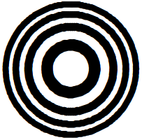
Figure \( 13.37\): A zone plate.