
3.4: Coulomb's Law


- Last updated
- Aug 27, 2023
- Save as PDF

( \newcommand{\kernel}{\mathrm{null}\,}\)
By the end of this section, you will be able to:
- State Coulomb’s law in terms of how the electrostatic force changes with the distance between two objects.
- Calculate the electrostatic force between two charged point forces, such as electrons or protons.
- Compare the electrostatic force to the gravitational attraction for a proton and an electron; for a human and the Earth.
Through the work of scientists in the late 18th century, the main features of the electrostatic force—the existence of two types of charge, the observation that like charges repel, unlike charges attract, and the decrease of force with distance—were eventually refined, and expressed as a mathematical formula. The mathematical formula for the electrostatic force is called Coulomb’s law after the French physicist Charles Coulomb (1736–1806), who performed experiments and first proposed a formula to calculate it.

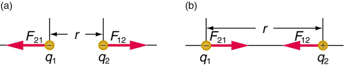
Coulomb’s law calculates the magnitude of the force F between two point charges, q1 and q2, separated by a distance r.
F=k|q1q2|r2.
In SI units, the constantk is equal to
k=8.988×10⁹N⋅m2C2≈8.99×10⁹N⋅m2C2.
The electrostatic force is a vector quantity and is expressed in units of newtons. The force is understood to be along the line joining the two charges. (Figure 3.4.2)
Although the formula for Coulomb’s law is simple, it was no mean task to prove it. The experiments Coulomb did, with the primitive equipment then available, were difficult. Modern experiments have verified Coulomb’s law to great precision. For example, it has been shown that the force is inversely proportional to distance between two objects squared (F∝1/r2) to an accuracy of 1 part in 1016. No exceptions have ever been found, even at the small distances within the atom.
Compare the electrostatic force between an electron and proton separated by 0.530×10⁻¹⁰m with the gravitational force between them. This distance is their average separation in a hydrogen atom.
- Strategy
-
To compare the two forces, we first compute the electrostatic force using Coulomb’s law, F=k|q1q2r2. We then calculate the gravitational force using Newton’s universal law of gravitation. Finally, we take a ratio to see how the forces compare in magnitude.
- Solution
-
Entering the given and known information about the charges and separation of the electron and proton into the expression of Coulomb’s law yields
F=k|q1q2|r2=(8.99×10⁹N⋅m2/C2)×(1.60×10−19C)(1.60×10−19C)(0.530×10−10m)2
Thus the Coulomb force is
F=8.19×10⁻⁸N.
The charges are opposite in sign, so this is an attractive force. This is a very large force for an electron—it would cause an acceleration of 8.99×10²²m/s2(verification is left as an end-of-section problem).The gravitational force is given by Newton’s law of gravitation as:
FG=GmMr2,
where G=6.67×10⁻¹¹N⋅m2/kg2. Here m and M represent the electron and proton masses, which can be found in the appendices. Entering values for the knowns yields
FG=(6.67×10⁻¹¹N⋅m2/kg2)×(9.11×10−31kg)(1.67×10−27kg)(0.530×10−10m)2=3.61×10−47N
This is also an attractive force, although it is traditionally shown as positive since gravitational force is always attractive. The ratio of the magnitude of the electrostatic force to gravitational force in this case is, thus,
FFG=2.27×1039.
- Discussion
-
This is a remarkably large ratio! Note that this will be the ratio of electrostatic force to gravitational force for an electron and a proton at any distance (taking the ratio before entering numerical values shows that the distance cancels). This ratio gives some indication of just how much larger the Coulomb force is than the gravitational force between two of the most common particles in nature.
As the example implies, gravitational force is completely negligible on a small scale, where the interactions of individual charged particles are important. On a large scale, such as between the Earth and a person, the reverse is true. Most objects are nearly electrically neutral, and so attractive and repulsive Coulomb forces nearly cancel. Gravitational force on a large scale dominates interactions between large objects because it is always attractive, while Coulomb forces tend to cancel.
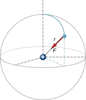
A hydrogen atom consists of a single proton and a single electron. The proton has a charge of +e and the electron has −e. In the “ground state” of the atom, the electron orbits the proton at most probable distance of 5.29×10⁻¹¹m (Figure 3.4.2). Calculate the electric force on the electron due to the proton.
- Strategy
-
For the purposes of this example, we are treating the electron and proton as two point particles, each with an electric charge, and we are told the distance between them; we are asked to calculate the force on the electron. We thus use Coulomb’s law (Equation ???).
- Answer
-
Our two charges are,
q1=+e=+1.602×10⁻¹⁹Cq2=−e=−1.602×10⁻¹⁹C
and the distance between them
r=5.29×10⁻¹¹m.
The magnitude of the force on the electron (Equation ???) is
F=14πϵ0|q1q2|r212=14π(8.85×10⁻¹²C2N⋅m2)(1.602×10⁻¹⁹C)2(5.29×10⁻¹¹m)2=8.25×10⁻⁸
As for the direction, since the charges on the two particles are opposite, the force is attractive; the force on the electron points radially directly toward the proton, everywhere in the electron’s orbit. The force is thus expressed as
→F=(8.25×10⁻⁸N)ˆr.
Multiple Source Charges
The analysis that we have done for two particles can be extended to an arbitrary number of particles; we simply repeat the analysis, two charges at a time. Specifically, we ask the question: Given N charges (which we refer to as source charge), what is the net electric force that they exert on some other point charge (which we call the test charge)?
Like all forces that we have seen up to now, the net electric force on our test charge is simply the vector sum of each individual electric force exerted on it by each of the individual test charges. Thus, we can calculate the net force on the test charge Q by calculating the force on it from each source charge, taken one at a time, and then adding all those forces together (as vectors). This ability to simply add up individual forces in this way is referred to as the principle of superposition, and is one of the more important features of the electric force. In mathematical form, this becomes
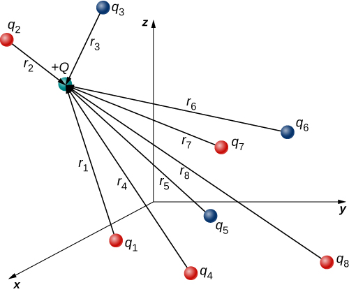
→F(r)=14πϵ0QN∑i=1qir2iˆri.
In this expression, Q represents the charge of the particle that is experiencing the electric force →F, and is located at →r from the origin; the q′is are the N source charges, and the vectors →ri are the displacements from the position of the ith charge to the position of Q. In the notation used for vector →ri, ri refers to the magnitude of the vector, and unit vector ˆri refers to its direction. Each of the N unit vectors points directly from its associated source charge toward the test charge. All of this is depicted in Figure 3.4.2. Please note that there is no physical difference between Q and qi; the difference in labels is merely to allow clear discussion, with Q being the charge we are determining the force on.
(Note that the force vector →Fi does not necessarily point in the same direction as the unit vector ˆri; it may point in the opposite direction, −ˆri. The signs of the source charge and test charge determine the direction of the force on the test charge.)
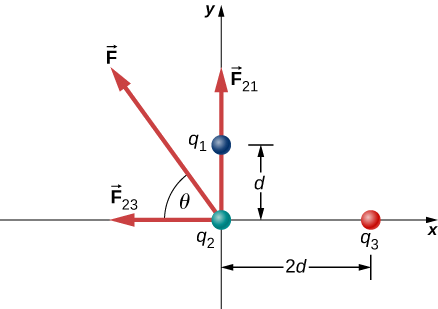
Three different, small charged objects are placed as shown in Figure 3.4.5. The charges q1 and q3 are fixed in place; q2 is free to move. Given q1=2e,q2=−3e, and q3=−5e, and that d=2.0×10⁻⁷m, what is the net force on the middle charge q2?
- Strategy
-
We use Coulomb’s law. The principle of superposition says that the force on q2 from each of the other charges is unaffected by the presence of the other charge. Therefore, we write down the force on q2 from each and add them together as vectors.
- Solution
-
We have two source charges q1 and q3 a test charge q2, distances r21 and r23 and we are asked to find a force. This calls for Coulomb’s law and superposition of forces. There are two forces:
→F=→F21+→F23.
x-component y-component →F21 F21x=0 F21y=14πϵ0[q2q1r221] →F23 F23x=14πϵ0[−q2q3r223] F23y=0 →F=→F21+→F23 Fx=F21x+F23x=14πϵ0[−q2q3r223] Fy=F21y+F23y=14πϵ0[q2q1r221] We cannot add these forces directly because they don’t point in the same direction: →F12 points only in the −x-direction, while →F13 points only in the +y-direction. The net force is obtained from applying the Pythagorean theorem to its x- and y-components:
F=√F2x+F2y
and
Fx=−F23=−14πϵ0q2q3r223=−(8.99×10⁹N⋅m2C2)(4.806×10⁻¹⁹C)(8.01×10⁻¹⁹C)(4.00×10⁻⁷m)2=−2.16×10⁻¹⁴N
and
Fy=F21=14πϵ0q2q1r21=(9.99×10⁹N⋅m2C2)(4.806×10⁻¹⁹C)(3.204×10⁻¹⁹C)(2.00×10⁻⁷m)2=3.46×10⁻¹⁴N.
We find that
F=√F2x+F2y=4.08×10⁻¹⁴N
at an angle of
ϕ=tan−1(FyFx)=tan−1(3.46×10⁻¹⁴N−2.16×10⁻¹⁴N)=−58o,
that is, 58o above the −x-axis, as shown in the diagram.
- Significance
-
Notice that when we substituted the numerical values of the charges, we did not include the negative sign of either q1 or q3. Recall that negative signs on vector quantities indicate a reversal of direction of the vector in question. But for electric forces, the direction of the force is determined by the types (signs) of both interacting charges; we determine the force directions by considering whether the signs of the two charges are the same or are opposite. If you also include negative signs from negative charges when you substitute numbers, you run the risk of mathematically reversing the direction of the force you are calculating. Thus, the safest thing to do is to calculate just the magnitude of the force, using the absolute values of the charges, and determine the directions physically.
It’s also worth noting that the only new concept in this example is how to calculate the electric forces; everything else (getting the net force from its components, breaking the forces into their components, finding the direction of the net force) is the same as force problems you have done earlier.
Summary
- Frenchman Charles Coulomb was the first to publish the mathematical equation that describes the electrostatic force between two objects.
- Coulomb’s law gives the magnitude of the force between point charges. It is F=k|q1q2|r2, where q1 and q2 are two point charges separated by a distance r, and k≈8.99×10⁹N⋅m2/C2
- This Coulomb force is extremely basic, since most charges are due to point-like particles. It is responsible for all electrostatic effects and underlies most macroscopic forces.
- The Coulomb force is extraordinarily strong compared with the gravitational force, another basic force—but unlike gravitational force it can cancel, since it can be either attractive or repulsive.
- The electrostatic force between two subatomic particles is far greater than the gravitational force between the same two particles.
Glossary
- Coulomb’s law
- the mathematical equation calculating the electrostatic force vector between two charged particles
- Coulomb force
- another term for the electrostatic force
- electrostatic force
- the amount and direction of attraction or repulsion between two charged bodies