2.5: Electric Fields and Forces with Multiple Charges

Learning Objectives

By the end of this section, you will be able to:

• Describe and apply the principle of superposition.
• Calculate the electric field of a set of source charges of either sign.

Principle of Superposition

Another experimental fact about the electric field is that it obeys the superposition principle. In this context, that means that we can (in principle) calculate the total electric field of many source charges by calculating the electric field of only \(q_1\) at a test position \(P\), then calculate the field of \(q_2\) at \(P\), while—and this is the crucial idea—ignoring the field of, and indeed even the existence of, \(q_1\). We can repeat this process, calculating the field of each individual source charge, independently of the existence of any of the other charges. The total electric field, then, is the vector sum of all these fields.

The Electric Field of Multiple Point Charges

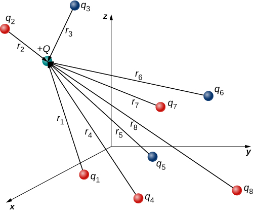
We next derive an equation that will allow us to perform the aforementioned calculation. Suppose we have \(N\) source charges \(q_1, q_2, q_3, . . . q_N\) located at positions \(\vec{r}_1, \vec{r}_2, \vec{r}_3, . . . \vec{r}_N\). By the principle of superposition, it follows from definition of the electric field that the net electric field is then

\[\vec{E} \equiv \dfrac{1}{4 \pi \epsilon_0}\left(\dfrac{q_1}{r_1^2}\hat{r}_1 + \dfrac{q_2}{r_2^2}\hat{r}_2 + \dfrac{q_3}{r_3^2}\hat{r}_3 + . . . + \dfrac{q_N}{r_1^2}\hat{r}_N\right) \label{Efield2} \]

or, more compactly,

\[\vec{E}(P) \equiv \dfrac{1}{4 \pi \epsilon_0} \sum_{i=1}^N \dfrac{q_i}{r_i^2}\hat{r}_i. \label{Efield3} \]

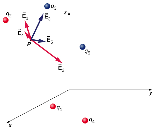
This expression is called the electric field at position \(P = P(x, y, z)\) of the \(N\) source charges. Here, \(P\) is the location of the point in space where you are calculating the field and is relative to the positions \(\vec{r}_i\) of the source charges (Figure \(\PageIndex{1}\)). Note that we have to impose a coordinate system to solve actual problems.

Figure \(\PageIndex{1}\): Each of these five source charges creates its own electric field at every point in space; shown here are the field vectors at an arbitrary point P. Like the electric force, the net electric field obeys the superposition principle.

Notice that the calculation of the electric field does not use the test charge. Thus, the physically useful approach is to calculate the electric field and then use it to calculate the force on some test charge later, if needed. Different test charges may experience different forces, but the same electric field exists at the test location by Equation \ref{Efield3}. That being said, recall that there is no fundamental difference between a test charge and a source charge; these are merely convenient labels for the system of interest. Any charge produces an electric field; however, just as Earth’s orbit is not affected by Earth’s own gravity, a charge is not subject to a force due to the electric field it generates. Charges are only subject to forces from the electric fields of other charges.

Examples \(\PageIndex{1A}\) and \(\PageIndex{1B}\) provide some examples of how to apply Equation \ref{Efield3}

Example \(\PageIndex{1A}\): The E-field of an Atom

In an ionized helium atom, the most probable distance between the nucleus and the electron is \(r = 26.5 \times 10^{-12}\ \textrm{m}\). What is the electric field due to the nucleus at the location of the electron?

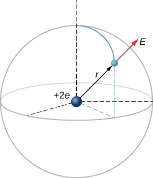
PLAN  Note that although the electron is mentioned, it is not used in any calculation. The problem asks for an electric field, not a force; hence, there is only one charge involved, and the problem specifically asks for the field due to the nucleus. Thus, only the distance of the electron matters. Also, since the distance between the two protons in the nucleus is much, much smaller than the distance of the electron from the nucleus, we can treat the two protons as a single charge +2\(e\).

SKETCH  

A diagram of the system is shown in Figure \(\PageIndex{2}\).

Figure \(\PageIndex{2}\): A schematic representation of a helium atom. Again, helium physically looks nothing like this, but this sort of diagram is helpful for calculating the electric field of the nucleus.

CALCULATE  The electric field is calculated by

\[\vec{E} = \dfrac{1}{4 \pi \epsilon_0} \sum_{i=1}^N \dfrac{q_i}{r_i^2} \hat{r}_i. \nonumber \]

Since there is only one source charge (the nucleus), this expression simplifies to

\[\vec{E} = \dfrac{1}{4\pi \epsilon_0}\dfrac{q}{r^2}\hat{r}. \nonumber \]

Here, \(q = 2e = 2(1.6 \times 10^{-19} \, \textrm{C})\) (since there are two protons) and \(r\) is given; substituting gives

\[ \begin{align*} \vec{E} &= \dfrac{1}{4\pi \left(8.85 \times 10^{-12} \dfrac{\textrm{C}^2}{\textrm{N}\cdot \textrm{m}^2}\right)} \dfrac{2(1.6 \times 10^{-19}\,\textrm{C})}{26.5 \times 10^{-12}\,\textrm{m})^2}\hat{r} \\[4pt] &= 4.1 \times 10^{12} \dfrac{\textrm{N}}{\textrm{C}}\hat{r}. \end{align*} \]

CHECK  The direction of \(\vec{E}\) is radially away from the nucleus in all directions. Why? Because a positive test charge placed in this field would accelerate radially away from the nucleus (since it is also positively charged), and again, the convention is that the direction of the electric field vector is defined in terms of the direction of the force it would apply to positive test charges.

Example \(\PageIndex{1B}\): The E-Field above Two Equal Charges

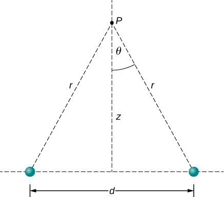
1. Find the electric field (magnitude and direction) a distance \(z\) above the midpoint between two equal charges \(+q\) that are a distance \(d\) apart (Figure \(\PageIndex{3}\)). Check that your result is consistent with what you would expect when \(z \gg d\).
2. Next, change the right-hand charge to \(-q\) instead of \(+q\). What is the electric field at the same location with this new configuration of charges?

Figure \(\PageIndex{3}\): Finding the field of two identical source charges at the point \(P\). The charges are separated by a distance \(d\) with perpendicular bisector passing through \(P\) at a distance z. Due to the symmetry, the net field at \(P\) is entirely vertical. (Notice that this is not true away from the midline between the charges.)

PLAN  We add the two fields as vectors, per Equation \ref{Efield3}. Notice that the system (and therefore the field) is symmetrical about the vertical axis; as a result, the horizontal components of the field vectors cancel. This simplifies the math. Also, we take care to express our final answer in terms of only quantities that are given in the original statement of the problem: \(q\), \(z\), \(d\), and constants \((\pi, \epsilon_0)\).

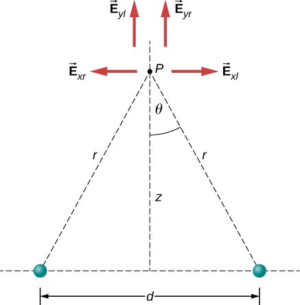
SKETCH   Figure \(\PageIndex{4}\) shows the charge configuration with the components of the electric field drawn in. 

Figure \(\PageIndex{4}\). Note that the horizontal components of the electric fields from the two charges cancel each other out, while the vertical components add together.

CALCULATE

a. By symmetry, the horizontal (\(x\))-components of \(\vec{E}\) cancel (Figure \(\PageIndex{4}\));

\[ \begin{align*} E_x &= \dfrac{1}{4\pi \epsilon_0} \dfrac{q}{r^2} \, \sin \, \theta - \dfrac{1}{4\pi \epsilon_0} \dfrac{q}{r^2} \, \sin \, \theta \\[4pt] &= 0. \end{align*} \]

The vertical (\(z\))-component is given by

\[ \begin{align*} E_z &= \dfrac{1}{4\pi \epsilon_0} \dfrac{q}{r^2} \, \cos \, \theta + \dfrac{1}{4\pi \epsilon_0} \dfrac{q}{r^2} \, \cos \, \theta \\[4pt] &= \dfrac{1}{4\pi \epsilon_0} \dfrac{2q}{r^2} \, \cos \, \theta. \end{align*} \]

Since none of the other components survive, this is the entire electric field, and it points in the \(\hat{k}\) direction. Notice that this calculation uses the principle of superposition; we calculate the fields of the two charges independently and then add them together.

What we want to do now is replace the quantities in this expression that we don’t know (such as \(r\)), or can’t easily measure (such as \(cos \, \theta\) with quantities that we do know, or can measure. In this case, by geometry,

\[r^2 = z^2 + \left(\dfrac{d}{2}\right)^2 \nonumber \]

and

\[\cos \, \theta = \dfrac{z}{R} = \dfrac{z}{\left[z^2 + \left(\dfrac{d}{2} \right)^2\right]^{1/2}}. \nonumber \]

Thus, substituting,

\[\vec{E}(z) = \dfrac{1}{4\pi \epsilon_0}\dfrac{2q}{\left[z^2 + \left(\dfrac{d}{2}\right)^2\right]^2} \dfrac{z}{\left[z^2 + \left(\dfrac{d}{2} \right)^2 \right]^{1/2}}\hat{k}. \nonumber \]

Simplifying, the desired answer is

\[\vec{E}(z) = \dfrac{1}{4\pi \epsilon_0}\dfrac{2qz}{\left[z^2 + \left(\dfrac{d}{2}\right)^2\right]^{3/2}} \hat{k}. \label{5.5} \]

b. If the source charges are equal and opposite, the vertical components cancel because

\[E_z = \dfrac{1}{4\pi \epsilon_0} \dfrac{q}{r^2} \, cos \, \theta - \dfrac{1}{4\pi \epsilon_0} \dfrac{q}{r^2} \, \cos \, \theta = 0 \nonumber \]

and we get, for the horizontal component of \(\vec{E}\).

\[\vec{E}(z) = \dfrac{1}{4\pi \epsilon_0} \dfrac{qd}{\left[z^2 + \left(\dfrac{d}{2}\right)^2\right]^{3/2}} \hat{i}.\label{5.6} \]

CHECK 

It is a very common and very useful technique in physics to check whether your answer is reasonable by evaluating it at extreme cases. In this example, we should evaluate the field expressions for the cases \(d = 0, \, z \gg d\), and \(z \rightarrow \infty\), and confirm that the resulting expressions match our physical expectations. Let’s do so:

Let’s start with Equation \ref{5.5}, the field of two identical charges. From far away (i.e., \(z >> d\)), the two source charges should “merge” and we should then “see” the field of just one charge, of size 2\(q\). So, let \(z \gg d\); then we can neglect \(d^2\) in Equation \ref{5.5} to obtain

\[ \begin{align*} \lim_{d\rightarrow 0}\vec{E} &= \dfrac{1}{4\pi \epsilon_0} \dfrac{2qz}{[z^2]^{3/2}}\hat{k} \\[4pt] &= \dfrac{1}{4\pi \epsilon_0} \dfrac{2qz}{z^3}\hat{k} \\[4pt] &= \dfrac{1}{4\pi \epsilon_0} \dfrac{2q}{z^2}\hat{k}, \end{align*} \]

which is the correct expression for a field at a distance \(z\) away from a charge \(2q\).

Next, we consider the field of equal and opposite charges, Equation \ref{5.6}. It can be shown (via a Taylor expansion) that for \(d \ll z \ll \infty\), , this becomes

\[\vec{E}(z) = \dfrac{1}{4\pi \epsilon_0} \dfrac{qd}{z^3}\hat{i}, \nonumber \]

which is the field of a dipole, a system that we will study in more detail later. (Note that the units of \(\vec{E}\) are still correct in this expression, since the units of \(d\) in the numerator cancel the unit of the “extra” \(z\) in the denominator.) If \(z\) is very large \((z \rightarrow \infty)\), then \(E \rightarrow 0\), as it should; the two charges “merge” and so cancel out.

Exercise \(\PageIndex{1}\)

Can you answer the questions in Example \(\PageIndex{1B}\) without using symmetry arguments? (Hint: Use Equation \ref{Efield3} and directly calculate the values of \hat{r}.)

Superposition of Electric Forces

Electric forces exerted by multiple charges also exhibit superposition.

Proof

Suppose we have \(N\) source charges \(q_1, q_2, q_3, . . . q_N\) located at positions \(\vec{r}_1, \vec{r}_2, \vec{r}_3, . . . \vec{r}_N\) along with a test charge \(Q\) at separate location (Fig. \(\PageIndex{5}\)). (Note that there is no physical difference between \(Q\) and \(q_i\); the difference in labels is merely to allow clear discussion, with \(Q\) being the charge we are determining the force on.)

Figure \(\PageIndex{5}\): In this example, the eight source ( \( N = 8 \) ) charges each apply a force on the single test charge Q. Each force can be calculated independently of the other seven forces. This is the essence of the superposition principle.

By Equation \ref{Efield3}, the net field at the test location of \(Q\) is

\[\vec{E_{net}}(P) = \dfrac{1}{4 \pi \epsilon_0} \sum_{i=1}^N \dfrac{q_i}{r_i^2}\hat{r}_i. \nonumber \]

From the definition of electric force,

\[ \begin{align*}
\vec{F}_{net} &= Q \vec{E}_{net} \\[4pt]
&= Q \left( \dfrac{1}{4 \pi \epsilon_0} \sum_{i=1}^N \dfrac{q_i}{r_i^2}\hat{r}_i \right) \\[4pt]
&= \left( \dfrac{1}{4 \pi \epsilon_0} \sum_{i=1}^N \dfrac{Q q_i}{r_i^2}\hat{r}_i \right) \\[4pt]
&= \left( \sum_{i=1}^N \vec{F}_i \right)
\end{align*} \]

Therefore, the electric force also obeys superposition.

There is a complication, however. Just as the source charges each exert a force on the test charge, so too (by Newton’s third law) does the test charge exert an equal and opposite force on each of the source charges. As a consequence, each source charge would change position. However, by the definition of electric force, the force on the test charge is a function of position; thus, as the positions of the source charges change, the net force on the test charge necessarily changes, which changes the force, which again changes the positions. Thus, the entire mathematical analysis quickly becomes intractable. Later, we will learn techniques for handling this situation, but for now, we make the simplifying assumption that the source charges are fixed in place, so that their positions are constant in time. (The test charge is allowed to move.) With this restriction in place, the analysis of charges is known as electrostatics, where “statics” refers to the constant (that is, static) positions of the source charges and the force is referred to as an electrostatic force.

Example \(\PageIndex{2}\): The Net Force from Two Source Charges

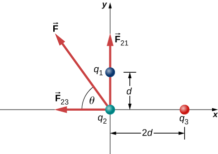
Three different, small charged objects are placed as shown in Figure \(\PageIndex{2}\). The charges \(q_1\) and \(q_3\) are fixed in place; \(q_2\) is free to move. Given \(q_1 = 2e, \, q_2 = -3e\), and \(q_3 = -5e\), and that \(d = 2.0 \times 10^{-7}\ \textrm{m}\), what is the net force on the middle charge \(q_2\)?

PLAN  

There are two possible approaches to this problem. One way would be to use Coulomb's law twice: once to calculate the electric force of \(q_1\) on \(q_2\) and again to calculate the electric force of \(q_3\) on \(q_2\). In this approach, \(q_2\) is our test charge, and \(q_1\) and \(q_3\) are source charges. Superposition of electric forces could then be used to add the two forces to find the net force on \(q_2\).

The other way would be to calculate the net electric field at the test location of \(q_2\) by using superposition of the electric fields due to \(q_1\) and \(q_2\). The net force can then be computed by using the definition of electric force to multiply the net electric field by the charge \(q_2\).

We will show solutions by both approaches.  In both approaches, we will model the small charged objects as point charges.

SKETCH  Figure \(\PageIndex{2}\) plots the locations of the charges.  We also draw the expected directions of the forces given the signs of the charges.

Figure \(\PageIndex{4}\): Source charges \(q_1\) and \(q_3\) each apply a force on \(q_2\).

Solution #1: Force Superposition

CALCULATE  We have two source charges \(q_1\) and \(q_3\) a test charge \(q_2\), distances \(r_{21}\) and \(r_{23}\) and we are asked to find a force. This calls for Coulomb’s law and superposition of forces. There are two forces:

\[\begin{align*} \vec{F} &= \vec{F}_{21} + \vec{F}_{23} = \dfrac{1}{4\pi \epsilon_0}\left[\dfrac{q_2q_1}{r_{21}^2}\hat{j} + \left(-\dfrac{q_2q_3}{r_{23}^2}\hat{i}\right)\right]. \end{align*}\]

We cannot add these forces directly because they don’t point in the same direction: \(\vec{F}_{12}\) points only in the \(-x\)-direction, while \(\vec{F}_{13}\) points only in the \(+y\)-direction. The net force is obtained from applying the Pythagorean theorem to its \(x\)- and \(y\)-components:

\[F = \sqrt{F_x^2 + F_y^2} \nonumber\]

and

\[\begin{align*} F_x &= -F_{23} = -\dfrac{1}{4\pi \epsilon_0} \dfrac{q_2q_3}{r_{23}^2} \\[4pt] &= - \left(8.99 \times 10^9 \dfrac{\textrm{N}\cdot \textrm{m}^2}{\textrm{C}^2}\right) \dfrac{(4.806 \times 10^{-19}\,\textrm{C})(8.01 \times 10^{-19}\,\textrm{C})}{(4.00 \times 10^{-7}\.\textrm{m})^2} \\[4pt] &= -2.16 \times 10^{-14} \,\textrm{N}\end{align*}\]

and

\[\begin{align*}F_y &= F_{21} = \dfrac{1}{4\pi \epsilon_0} \dfrac{q_2q_1}{r_{21}} \\[4pt] &= \left(8.99 \times 10^9 \dfrac{N \cdot m^2}{C^2}\right) \dfrac{(4.806 \times 10^{-19}C)(3.204 \times 10^{-19}C)}{(2.00 \times 10^{-7} m)^2} \\[4pt] &= 3.45 \times 10^{-14} \, N.\end{align*}\]

We find that

\[\begin{align*} F &= \sqrt{F_x^2 + F_y^2} \\[4pt] &= 4.07 \times 10^{-14} \,\textrm{N} \end{align*}\]

at an angle of

\[\begin{align*} \phi &= \tan^{-1} \left(\dfrac{F_y}{F_x}\right) \\[4pt] &= \tan^{-1} \left( \dfrac{3.46 \times 10^{-14} N}{-2.16 \times 10^{-14}N} \right) \\[4pt] &= -58^\circ, \end{align*}\]

that is, \(58^\circ\) above the \(-x\)-axis, as shown in the diagram.

CHECK  Notice that when we substituted the numerical values of the charges, we did not include the negative sign of either \(q_1\) or \(q_3\). Recall that negative signs on vector quantities indicate a reversal of direction of the vector in question. But for electric forces, the direction of the force is determined by the types (signs) of both interacting charges; we determine the force directions by considering whether the signs of the two charges are the same or are opposite. If you also include negative signs from negative charges when you substitute numbers, you run the risk of mathematically reversing the direction of the force you are calculating. Thus, the safest thing to do is to calculate just the magnitude of the force, using the absolute values of the charges, and determine the directions physically.

It is also worth noting that the only new concept in this example is how to calculate the electric forces; everything else (getting the net force from its components, breaking the forces into their components, finding the direction of the net force) is the same as force problems you have done earlier.

Solution #2: Field Superposition

CALCULATE  First, calculate the electric field due to \(q_1\) at the test location of \(q_2\). We identify the location of the source charge as \( (x_s, y_s) = (0, d) \) and the test location as \( (x_t, y_t) = (0, 0) \). As a result,

\[ \begin{align*}
\Delta x &= x_t - x_s = 0 - 0 = 0,\\
\Delta y &= y_t - y_s = 0 - d = -d, \\
\end{align*} \]

and therefore the separation distance is given by

\[ r = [(\Delta x)^2 + (\Delta y)^2 ]^{1/2} = [(0)^2 + (-d)^2]^{1/2} = d . \nonumber \]

The radial unit vector is then given by

\[ \hat{r} = \dfrac{(\Delta x)\hat{i}+(\Delta y)\hat{j}}{[(\Delta x)^2 + (\Delta y)^2]^{1/2}}
= \dfrac{(0)\hat{i}+(-d)\hat{j}}{d}
= -\hat{j}.
\nonumber \]

The electric field at the test location is then given by

\[ \vec{E}_1 = k_e \dfrac{q_1}{r^2}\hat{r} = k_e \dfrac{2e}{d^2}(-\hat{j}) \nonumber \]

Next, calculate the electric field due to \(q_3\) at the test location of \(q_2\). We identify the location of the source charge as \( (x_s, y_s) = (2d, 0) \) and the test location as \( (x_t, y_t) = (0, 0) \). As a result,

\[ \begin{align*}
\Delta x &= x_t - x_s = 0 - 2d = -2d,\\
\Delta y &= y_t - y_s = 0 - 0 = 0, \\
\end{align*} \]

and therefore the separation distance is given by

\[ r = [(\Delta x)^2 + (\Delta y)^2 ]^{1/2} = [(2d)^2 + (0)^2]^{1/2} = 2d . \nonumber \]

The radial unit vector is then given by

\[ \hat{r} = \dfrac{(\Delta x)\hat{i}+(\Delta y)\hat{j}}{[(\Delta x)^2 + (\Delta y)^2]^{1/2}}
= \dfrac{(-2d)\hat{i}+(0)\hat{j}}{2d}
= -\hat{i}.
\nonumber \]

The electric field at the test location is then given by

\[ \vec{E}_3 = k_e \dfrac{q_3}{r^2}\hat{r} = k_e \dfrac{-5e}{(2d)^2}(-\hat{i}) \nonumber \]

The net electric field is

\[ \vec{E}_{net} = \vec{E}_1 + \vec{E}_3 = k_e \dfrac{e}{d^2} ( -2\hat{j} + 1.25\hat{i} ) \]

The net electric force is then
\[ \begin{align*}
\vec{F}_{net} &= q_2 \vec{E}_{net} \\[4pt]
&= (-3e)\left[ k_e \dfrac{e}{d^2} ( -2\hat{j} + 1.25\hat{i} ) \right] \\[4pt]
&= k_e \dfrac{e^2}{d^2} ( 6\hat{j}-3.75\hat{i} ) \\[4pt]
&= \left( 8.99 \times 10^9 \dfrac{\mathrm{N}\cdot \mathrm{m}^2}{\mathrm{C}^2} \right)
\dfrac{(1.6\times 10^{-19}\ \mathrm{C})^2}{(2.0\times 10^{-7}\ \mathrm{m})^2}(-3.75\hat{i} + 6\hat{j})\\[4pt]
&= (-2.16 \times 10^{-14}\ \mathrm{N}) \hat{i} + (3.45\times 10^{-14}\ \mathrm{N}) \hat{j}
\end{align*} \]

This value is the same result as in Solution #1.

CHECK  While the second approach may take a bit more math, it has the advantage of following a systematic method of calculation. You do not necessarily have to think separately about which directions the fields are going; these directions automatically come out of the calculation of the products of the source charges with the radial unit vectors. The force calculation is somewhat simpler because you only have to multiply the test charge by the net electric field once.

It is reassuring that both methods give the same result!

Exercise \(\PageIndex{2}\)

What would be different in Example \(\PageIndex{2}\) if \(q_1\) were negative rather than positive?

Answer

The net force would point \(58^\circ\) below the −\(x\)-axis.

As suggested above, a charge that is not held in place will move under the influence of electric forces. By solving the equations of motion with a computer, it is possible to calculate the path of the charge's motion.

PhET Simulation: Electric Field Hockey

The goal of the game of "Electric Field Hockey" is to get the positively-charged puck in the goal by placing other charges in fixed locations on the field.

Instructions:

1. Click on the link to open a new browser window containing the simulation.
2. Click on the arrow in the center of the simulation.
3. In the resulting dialog box, select "Run CheerpJ Browser-Compatible Version" to run the Java simulation in your browser.
4. Place positive and negative charges on to the field in a way that you think will attract or repel the positively-charged puck.
5. Select the "Trace" checkbox to show the path of the puck as it travels.
6. Press "Start" to begin the simulation.
7. If the puck goes into the goal, you win. If it does not go into the goal, press the "Reset" button.
8. If you need some guidance, turn on the electric field display by selecting the "Field" checkbox.
9. At each level of difficulty, you should strive to use as few positive and negative charges as possible to score a goal.

Source: Electric Field Hockey

Simulation by PhET Interactive Simulations, University of Colorado Boulder, licensed under CC-BY-4.0 (opens in new window).