5.8: Common Forces - The Coulomb Force

Learning Objectives

By the end of this section, you will be able to:

• Describe the electric force, both qualitatively and quantitatively
• Calculate the force that charges exert on each other

Experiments with electric charges have shown that if two objects each have electric charge, then they exert an electric force on each other. The magnitude of the force is linearly proportional to the net charge on each object and inversely proportional to the square of the distance between them. The direction of the force vector is along the imaginary line joining the two objects and is dictated by the signs of the charges involved.

Let

• \(q_1, q_2 =\) the net electric charge of the two objects;
• \(\vec{r}_{12} =\) the vector displacement from \(q_1\) to \(q_2\).

The electric force \(\vec{F}\) on one of the charges is proportional to the magnitude of its own charge and the magnitude of the other charge, and is inversely proportional to the square of the distance between them:

\[F \propto \dfrac{q_1q_2}{r_{12}^2}.\]

This proportionality becomes an equality with the introduction of a proportionality constant. For reasons that will become clear in a later chapter, the proportionality constant that we use is actually a collection of constants. (We discuss this constant shortly.)

Coulomb's Law

The magnitude of the electric force (or Coulomb force) between two electrically charged particles is equal to

\[\left|\mathbf{F}_{12}\right|=\frac{1}{4 \pi \varepsilon_{0}} \frac{\left|q_{1} q_{2}\right|}{r_{12}^{2}} \label{Coulomb}\]

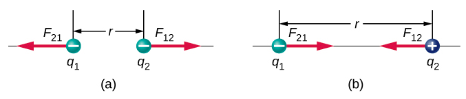
The unit vector \(r\) has a magnitude of 1 and points along the axis as the charges. If the charges have the same sign, the force is in the same direction as \(r\) showing a repelling force. If the charges have different signs, the force is in the opposite direction of \(r\) showing an attracting force. (Figure \(\PageIndex{1}\)).

Figure \(\PageIndex{1}\): The electrostatic force \(\vec{F}\) between point charges \(q_1\) and \(q_2\) separated by a distance \(r\) is given by Coulomb’s law. Note that Newton’s third law (every force exerted creates an equal and opposite force) applies as usual—the force on \(q_1\) is equal in magnitude and opposite in direction to the force it exerts on \(q_2\). (a) Like charges; (b) unlike charges.

It is important to note that the electric force is not constant; it is a function of the separation distance between the two charges. If either the test charge or the source charge (or both) move, then \(\vec{r}\) changes, and therefore so does the force. An immediate consequence of this is that direct application of Newton’s laws with this force can be mathematically difficult, depending on the specific problem at hand. It can (usually) be done, but we almost always look for easier methods of calculating whatever physical quantity we are interested in. (Conservation of energy is the most common choice.)

Finally, the new constant \(\epsilon_0\) in Coulomb’s law is called the permittivity of free space, or (better) the permittivity of vacuum. It has a very important physical meaning that we will discuss in a later chapter; for now, it is simply an empirical proportionality constant. Its numerical value (to three significant figures) turns out to be

\[\epsilon_0 = 8.85 \times 10^{-12} \dfrac{C^2}{N \cdot m^2}.\]

These units are required to give the force in Coulomb’s law the correct units of newtons. Note that in Coulomb’s law, the permittivity of vacuum is only part of the proportionality constant. For convenience, we often define a Coulomb’s constant:

\[k_e = \dfrac{1}{4\pi \epsilon_0} = 8.99 \times 10^9 \dfrac{N \cdot m^2}{C^2}.\]

Example \(\PageIndex{1}\): The Force on the Electron in Hydrogen

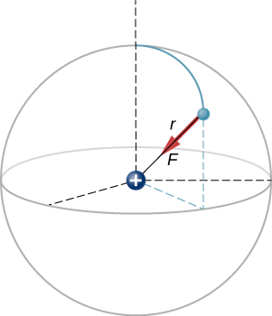
A hydrogen atom consists of a single proton and a single electron. The proton has a charge of \(+e\) and the electron has \(-e\). In the “ground state” of the atom, the electron orbits the proton at most probable distance of \(5.29 \times 10^{-11} m\) (Figure \(\PageIndex{2}\)). Calculate the electric force on the electron due to the proton.

Figure \(\PageIndex{2}\): A schematic depiction of a hydrogen atom, showing the force on the electron. This depiction is only to enable us to calculate the force; the hydrogen atom does not really look like this.

Strategy

For the purposes of this example, we are treating the electron and proton as two point particles, each with an electric charge, and we are told the distance between them; we are asked to calculate the force on the electron. We thus use Coulomb’s law (Equation \ref{Coulomb}).

Solution

Our two charges are,

\[\begin{align*} q_1 &= +e \\[4pt] &= +1.602 \times 10^{-19} C \\[4pt] q_2 &= -e \\[4pt] &= -1.602 \times 10^{-19} C \end{align*}\]

and the distance between them

\[r = 5.29 \times 10^{-11} m. \nonumber\]

The magnitude of the force on the electron (Equation \ref{Coulomb}) is

\[\begin{align*} F &= \dfrac{1}{4\pi \epsilon_0}\dfrac{|q_1q_2|}{r_{12}^2} \\[4pt] &= \dfrac{1}{4\pi \left(8.85 \times 10^{-12} \frac{C^2}{N \cdot m^2} \right)} \dfrac{(1.602 \times 10^{-19} C)^2}{(5.29 \times 10^{-11} m)^2} \\[4pt] &= 8.25 \times 10^{-8} \end{align*}\]

As for the direction, since the charges on the two particles are opposite, the force is attractive; the force on the electron points radially directly toward the proton, everywhere in the electron’s orbit. The force is thus expressed as

\[\vec{F} = (8.25 \times 10^{-8} N) \hat{r}. \nonumber\]

Significance

This is a three-dimensional system, so the electron (and therefore the force on it) can be anywhere in an imaginary spherical shell around the proton. In this “classical” model of the hydrogen atom, the electrostatic force on the electron points in the inward centripetal direction, thus maintaining the electron’s orbit. But note that the quantum mechanical model of hydrogen (discussed in Quantum Mechanics) is utterly different.