20.3: Examples

Whiteboard Problem \(\PageIndex{1}\): Seesaw

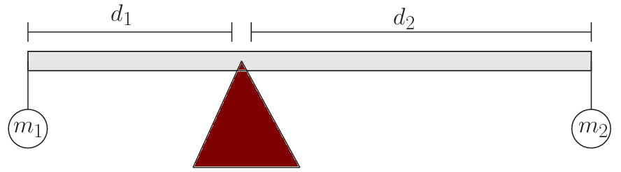
Consider the see-saw in the above figure - two masses attached to a massless board, balanced on a point between them.

1. If \(d_1\) = 37.5 cm, \(d_2\) = 113 cm, and \(m_1\) = 15 kg, what should \(m_2\) be so that this board is balanced?
2. How much force is the balance point acting on the board with?

Whiteboard Problem \(\PageIndex{2}\): Steel Beam

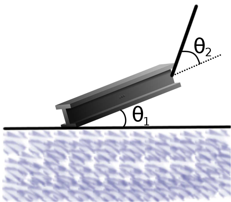
Consider the steel beam shown in the figure, with a mass of 2450 kg, being held in place by a crane. The angle between the horizontal and the beam is 15\(^\circ\), and the angle between the axis of the beam and the cable is 63\(^\circ\).

1. What is the tension in the cable, if the length of the beam is 6.5 m?
2. How much force, and in which direction, is the ground acting on the beam with?

Whiteboard Problem \(\PageIndex{3}\): Sliding Penguin

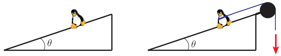
Consider a penguin sitting on a ramp, as shown in the figure on the left. The ramp makes an angle of 15\(^\circ\) with respect to the floor, the mass of the penguin is 45 kg, and the coefficient of static friction between the penguin and the ramp is 0.30.

1. If the penguin is not moving, how large is the frictional force acting on it?
2. Now I tie a rope to the penguin, as shown in the figure on the right. This rope goes over a frictionless, massless pulley. How hard must I pull on the rope before the penguin just starts to move?

Whiteboard Problem \(\PageIndex{4}\): Sliding Penguin Reduex

Consider a penguin sitting on a ramp as shown in the lefthand figure for Whiteboard Problem \(\PageIndex{3}\) (without the rope). This is an Emperor Penguin, so naturally it has a mass of 45 kg.

1. If the coefficient of static friction between the ramp and the penguin is 0.40, what is the maximum angle the ramp can have if the penguin is going to remain stationary?
2. If I increase the angle a little bit from part (a) then penguin will start to slide. Say I increase this angle by 10\%, and the coefficient of kinetic friction between the penguin and the ramp is 0.30, what will the acceleration of the penguin be?

Whiteboard Problem \(\PageIndex{5}\): Curling for Torque!

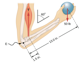
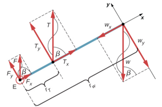
A weightlifter is holding a 50.0-lb weight (equivalent to 222.4 N) with his forearm, as shown in the Figure. His forearm is positioned at \(\theta = 60^\circ\) with respect to his upper arm, and supported by the biceps muscle, which causes a torque around the elbow (labeled ``E''). You can assume the tension $T$ on the bicep muscle is directed straight up, opposite the direction of gravity, and you can ignore the weight of the arm.

1. What tension force is in the bicep muscle? (That is, ``find \(T\)''!)
2. What is the magnitude of the force at the elbow joint?
3. In what direction (describe or find an angle!) is the force at the elbow joint acting?

Note: this problem came from the Open Stax textbook University Physics Volume 1, and they solve it there using the following free body diagram. You are welcome to do that as well - but do you think that coordinate system is the best choice?

Learning Objectives

• Identify and analyze static equilibrium situations
• Set up a free-body diagram for an extended object in static equilibrium
• Set up and solve static equilibrium conditions for objects in equilibrium in various physical situations

All examples in this chapter are planar problems. Accordingly, we use equilibrium conditions in the component form of Equation 12.2.9 to Equation 12.2.11. We introduced a problem-solving strategy in Example 12.1 to illustrate the physical meaning of the equilibrium conditions. Now we generalize this strategy in a list of steps to follow when solving static equilibrium problems for extended rigid bodies. We proceed in five practical steps.

Problem-Solving Strategy: Static Equilibrium

1. Identify the object to be analyzed. For some systems in equilibrium, it may be necessary to consider more than one object. Identify all forces acting on the object. Identify the questions you need to answer. Identify the information given in the problem. In realistic problems, some key information may be implicit in the situation rather than provided explicitly.
2. Set up a free-body diagram for the object. (a) Choose the xy-reference frame for the problem. Draw a free-body diagram for the object, including only the forces that act on it. When suitable, represent the forces in terms of their components in the chosen reference frame. As you do this for each force, cross out the original force so that you do not erroneously include the same force twice in equations. Label all forces—you will need this for correct computations of net forces in the x- and y-directions. For an unknown force, the direction must be assigned arbitrarily; think of it as a ‘working direction’ or ‘suspected direction.’ The correct direction is determined by the sign that you obtain in the final solution. A plus sign (+) means that the working direction is the actual direction. A minus sign (−) means that the actual direction is opposite to the assumed working direction. (b) Choose the location of the rotation axis; in other words, choose the pivot point with respect to which you will compute torques of acting forces. On the free-body diagram, indicate the location of the pivot and the lever arms of acting forces—you will need this for correct computations of torques. In the selection of the pivot, keep in mind that the pivot can be placed anywhere you wish, but the guiding principle is that the best choice will simplify as much as possible the calculation of the net torque along the rotation axis.
3. Set up the equations of equilibrium for the object. (a) Use the free-body diagram to write a correct equilibrium condition Equation 12.2.9 for force components in the x-direction. (b) Use the free-body diagram to write a correct equilibrium condition Equation 12.2.13 for force components in the y-direction. (c) Use the free-body diagram to write a correct equilibrium condition Equation 12.2.11 for torques along the axis of rotation. Use Equation 12.2.12 to evaluate torque magnitudes and senses.
4. Simplify and solve the system of equations for equilibrium to obtain unknown quantities. At this point, your work involves algebra only. Keep in mind that the number of equations must be the same as the number of unknowns. If the number of unknowns is larger than the number of equations, the problem cannot be solved.
5. Evaluate the expressions for the unknown quantities that you obtained in your solution. Your final answers should have correct numerical values and correct physical units. If they do not, then use the previous steps to track back a mistake to its origin and correct it. Also, you may independently check for your numerical answers by shifting the pivot to a different location and solving the problem again, which is what we did in Example 12.1.

Note that setting up a free-body diagram for a rigid-body equilibrium problem is the most important component in the solution process. Without the correct setup and a correct diagram, you will not be able to write down correct conditions for equilibrium. Also note that a free-body diagram for an extended rigid body that may undergo rotational motion is different from a free-body diagram for a body that experiences only translational motion (as you saw in the chapters on Newton’s laws of motion). In translational dynamics, a body is represented as its CM, where all forces on the body are attached and no torques appear. This does not hold true in rotational dynamics, where an extended rigid body cannot be represented by one point alone. The reason for this is that in analyzing rotation, we must identify torques acting on the body, and torque depends both on the acting force and on its lever arm. Here, the free-body diagram for an extended rigid body helps us identify external torques.

Example \(\PageIndex{6}\): The Torque Balance

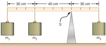
Three masses are attached to a uniform meter stick, as shown in Figure \(\PageIndex{1}\). The mass of the meter stick is 150.0 g and the masses to the left of the fulcrum are m₁ = 50.0 g and m₂ = 75.0 g. Find the mass m3 that balances the system when it is attached at the right end of the stick, and the normal reaction force at the fulcrum when the system is balanced.

Figure \(\PageIndex{1}\): In a torque balance, a horizontal beam is supported at a fulcrum (indicated by S) and masses are attached to both sides of the fulcrum. The system is in static equilibrium when the beam does not rotate. It is balanced when the beam remains level.

Strategy

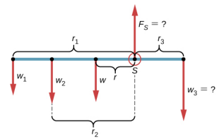
For the arrangement shown in the figure, we identify the following five forces acting on the meter stick:

1. w₁ = m₁g is the weight of mass m₁;
2. w₂ = m₂g is the weight of mass m₂;
3. w = mg is the weight of the entire meter stick;
4. w₃ = m₃g is the weight of unknown mass m₃;
5. F_S is the normal reaction force at the support point S.

We choose a frame of reference where the direction of the y-axis is the direction of gravity, the direction of the xaxis is along the meter stick, and the axis of rotation (the z-axis) is perpendicular to the x-axis and passes through the support point S. In other words, we choose the pivot at the point where the meter stick touches the support. This is a natural choice for the pivot because this point does not move as the stick rotates. Now we are ready to set up the free-body diagram for the meter stick. We indicate the pivot and attach five vectors representing the five forces along the line representing the meter stick, locating the forces with respect to the pivot Figure \(\PageIndex{2}\). At this stage, we can identify the lever arms of the five forces given the information provided in the problem. For the three hanging masses, the problem is explicit about their locations along the stick, but the information about the location of the weight w is given implicitly. The key word here is “uniform.” We know from our previous studies that the CM of a uniform stick is located at its midpoint, so this is where we attach the weight w, at the 50-cm mark.

Figure \(\PageIndex{2}\): Free-body diagram for the meter stick. The pivot is chosen at the support point S.

Solution

With Figure \(\PageIndex{1}\) and Figure \(\PageIndex{2}\) for reference, we begin by finding the lever arms of the five forces acting on the stick:

\[\begin{split} r_{1} & = 30.0\; cm + 40.0\; cm = 70.0\; cm \\ r_{2} & = 40.0\; cm \\ r & = 50.0\; cm - 30.0\; cm = 20.0\; cm \\ r_{S} & = 0.0\; cm\; (because\; F_{S}\; is\; attached\; at\; the\; pivot) \\ r_{3} & = 30.0\; cm \ldotp \end{split}\]

Now we can find the five torques with respect to the chosen pivot:

\[\begin{split} \tau_{1} & = +r_{1} w_{1} \sin 90^{o} = +r_{1} m_{1} g \quad (counterclockwise\; rotation,\; positive\; sense) \\ \tau_{2} & = +r_{2} w_{2} \sin 90^{o} = +r_{2} m_{2} g \quad (counterclockwise\; rotation,\; positive\; sense) \\ \tau & = +rw \sin 90^{o} = +rmg \quad \quad \quad (gravitational\; torque) \\ \tau_{S} & = r_{S} F_{S} \sin \theta_{S} = 0 \quad \quad \quad \quad \quad (because\; r_{S} = 0\; cm) \\ \tau_{3} & = -r_{3} w_{3} \sin 90^{o} = -r_{3} m_{3} g \quad (counterclockwise\; rotation,\; negative\; sense) \end{split}\]

The second equilibrium condition (equation for the torques) for the meter stick is

\[\tau_{1} + \tau_{2} + \tau + \tau_{S} + \tau_{3} = 0 \ldotp\]

When substituting torque values into this equation, we can omit the torques giving zero contributions. In this way the second equilibrium condition is

\[+r_{1} m_{1} g + r_{2} m_{2} g + rmg - r_{3} m_{3} g = 0 \ldotp \label{12.17}\]

Selecting the +y-direction to be parallel to \(\vec{F}_{S}\), the first equilibrium condition for the stick is

\[-w_{1} - w_{2} - w + F_{S} - w_{3} = 0 \ldotp\]

Substituting the forces, the first equilibrium condition becomes

\[-m_{1} g - m_{2} g - mg + F_{S} - m_{3} g = 0 \ldotp \label{12.18}\]

We solve these equations simultaneously for the unknown values m₃ and F_S. In Equation \ref{12.17}, we cancel the g factor and rearrange the terms to obtain

\[r_{3} m_{3} = r_{1} m_{1} + r_{2} m_{2} + rm \ldotp\]

To obtain m₃ we divide both sides by r₃, so we have

\[\begin{split} m_{3} & = \frac{r_{1}}{r_{3}} m_{1} + \frac{r_{2}}{r_{3}} m_{2} + \frac{r}{r_{3}} m \\ & = \frac{70}{30} (50.0\; g) + \frac{40}{30} (75.0\; g) + \frac{20}{30} (150.0\; g) = 315.0 \left(\dfrac{2}{3}\right)\; g \simeq 317\; g \ldotp \end{split} \label{12.19}\]

To find the normal reaction force, we rearrange the terms in Equation \ref{12.18}, converting grams to kilograms:

\[\begin{split} F_{S} & = (m_{1} + m_{2} + m + m_{3}) g \\ & = (50.0 + 75.0 + 150.0 + 316.7) \times (10^{-3}\; kg) \times (9.8\; m/s^{2}) = 5.8\; N \ldotp \end{split} \label{12.20}\]

Significance

Notice that Equation \ref{12.17} is independent of the value of g. The torque balance may therefore be used to measure mass, since variations in g-values on Earth’s surface do not affect these measurements. This is not the case for a spring balance because it measures the force.

Exercise \(\PageIndex{7}\)

Repeat Example 12.3 using the left end of the meter stick to calculate the torques; that is, by placing the pivot at the left end of the meter stick.

In the next example, we show how to use the first equilibrium condition (equation for forces) in the vector form given by Equation 12.2.9 and Equation 12.2.10. We present this solution to illustrate the importance of a suitable choice of reference frame. Although all inertial reference frames are equivalent and numerical solutions obtained in one frame are the same as in any other, an unsuitable choice of reference frame can make the solution quite lengthy and convoluted, whereas a wise choice of reference frame makes the solution straightforward. We show this in the equivalent solution to the same problem. This particular example illustrates an application of static equilibrium to biomechanics.

Exercise \(\PageIndex{8}\)

Repeat Example 12.4 assuming that the forearm is an object of uniform density that weighs 8.896 N.

Exercise \(\PageIndex{10}\)

Exercise \(\PageIndex{11}\)

Solve the problem in Example 12.6 by taking the pivot position at the center of mass.

Exercise \(\PageIndex{12}\)

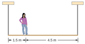
A 50-kg person stands 1.5 m away from one end of a uniform 6.0-m-long scaffold of mass 70.0 kg. Find the tensions in the two vertical ropes supporting the scaffold.

Exercise \(\PageIndex{13}\)

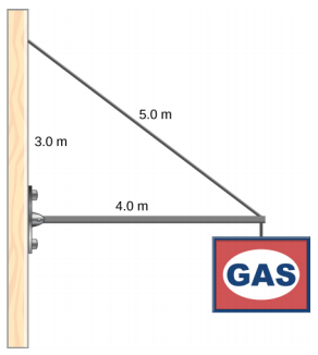
A 400.0-N sign hangs from the end of a uniform strut. The strut is 4.0 m long and weighs 600.0 N. The strut is supported by a hinge at the wall and by a cable whose other end is tied to the wall at a point 3.0 m above the left end of the strut. Find the tension in the supporting cable and the force of the hinge on the strut.

Example \(\PageIndex{14}\): A Simple Spring Problem

Consider a spring of unknown spring constant. You first want to find out what the spring constant actually is, and then use the spring to determine the mass of an unknown object. To do this, first you measure the equilibrium length of the spring to be 10 cm. Then, you put a mass of 5 kg on the end, hang it vertically, and observe that the spring stretches to a total length of 12 cm. What is the spring constant?

Now that you know the spring constant, you put the unknown mass on the spring and notice that it stretches to a length of 17 cm. What is the mass of this object?

Solution

1. Translate: We will use the following variables:
   \[y_0=10 \text{ cm},\quad y_1=12\text{ cm},\quad y_2=17\text{ cm},m_1=5\text{ kg},\quad m_2=?.\]
   Notice that we are not specifying the coordinate system quite yet - since the spring is hanging vertically, the y-coordinate might end up being negative. These are just the lengths of the various quantities we measured.
2. Model: Since the only thing we know about this system are lengths and masses, we are clearly going to have to use Hooke's law, \(F_{sp,y}=-k(y-y_0)\) (in the y-direction). Since this spring is hanging vertically, it makes sense to use Newton's 2nd law to model the equilbrium situation.
3. Solve: First, we write the condition for equilbrium when the known mass is hung on the spring. Here, we are going to take the vertical direction to be the y-coordinate, with positive upwards.
   \[\Sigma F_y = 0\rightarrow F_{sp,y}+F_{g,y}=0\rightarrow -k((-y_1)-(-y_0))+m_1g(-y_1)=0\rightarrow k=\frac{m_1gy_1}{y_1-y_0}\simeq 294\text{ Nm}\]
   Notice carefully what we did with the coordinates - we made all of them negative, with the top of the spring being the origin. Also take care that you do the conversions from centimeters to meters in the final calculation!
   Now that we have the spring constant, we can do the same thing for the unknown mass. This equation is going to look very similar, but switching around our known and unknown variables:
   \[\Sigma F_y = 0\rightarrow F_{sp,y}+F_{g,y}=0\rightarrow -k((-y_2)-(-y_0))+m_2g(-y_2)=0\rightarrow m_2=\frac{k(y_2-y_0)}{gy_2}\simeq 12.4\text {kg}.\]
   Again, take careful note of what happens algebraically with the signs.
4. Check: This is consistent with our intuition - the spring stretched more for a heavier mass. Since the amount of stretching was 5 cm as compared to 2 cm, we would expect that the mass is also more then twice as big, which it is!

Notice that although the stretching length was exactly 3.5 times bigger (7 cm / 2 cm = 3.5), the unknown mass was not 3.5 times bigger: 3.5*5 kg = 17.5 kg. We can see why this happens by using the last formula we wrote down, but plugging in the equation for the spring constant we found in the first part:

\[m_2=\frac{k(y_2-y_0)}{gy_2}=\left(\frac{m_1gy_1}{y_1-y_0} \right)\left(\frac{(y_2-y_0)}{gy_2}\right)=\left(\frac{y_1}{y_2}\right)\left(\frac{y_2-y_0}{y_1-y_0}\right)m_1.\]

So, the ratio between \(m_1\) and \(m_2\) is not simply the ratio of the displacements \((y_2-y_0)/(y_1-y_0)\), but is also scaled by the ratio of the stretch, \(y_1/y_2\).