The Carnot Cycle
- Last updated
- Jun 17, 2019
- Save as PDF
- Page ID
- 18075
( \newcommand{\kernel}{\mathrm{null}\,}\)
Learning Objectives
By the end of this section you will be able to:
- Describe the Carnot cycle with the roles of all four processes involved
- Outline the Carnot principle and its implications
- Demonstrate the equivalence of the Carnot principle and the second law of thermodynamics
In the early 1820s, Sadi Carnot (1786−1832), a French engineer, became interested in improving the efficiencies of practical heat engines. In 1824, his studies led him to propose a hypothetical working cycle with the highest possible efficiency between the same two reservoirs, known now as the Carnot cycle. An engine operating in this cycle is called a Carnot engine. The Carnot cycle is of special importance for a variety of reasons. At a practical level, this cycle represents a reversible model for the steam power plant and the refrigerator or heat pump. Yet, it is also very important theoretically, for it plays a major role in the development of another important statement of the second law of thermodynamics. Finally, because only two reservoirs are involved in its operation, it can be used along with the second law of thermodynamics to define an absolute temperature scale that is truly independent of any substance used for temperature measurement.

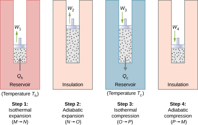
With an ideal gas as the working substance, the steps of the Carnot cycle, as represented by Figure 1, are as follows.
- Isothermal expansion. The gas is placed in thermal contact with a heat reservoir at a temperature Th. The gas absorbs heat Qh from the heat reservoir and is allowed to expand isothermally, doing work W1. Because the internal energy Eint of an ideal gas is a function of the temperature only, the change of the internal energy is zero, that is, ΔEint=0 during this isothermal expansion. With the first law of thermodynamics, ΔEint=Q−W, we find that the heat absorbed by the gas is Qh=W1=nRThlnVNVM.
- Adiabatic expansion. The gas is thermally isolated and allowed to expand further, doing work W2. Because this expansion is adiabatic, the temperature of the gas falls—in this case, from Th to Tc. From pVγ=constant and the equation of state for an ideal gas, pV=nRT, we have TVγ−1=constant, so that ThVγ−1N=TcVγ−1O.
- Isothermal compression. The gas is placed in thermal contact with a cold reservoir at temperature Tc and compressed isothermally. During this process, work W3 is done on the gas and it gives up heat Qc to the cold reservoir. The reasoning used in step 1 now yields Qc=nRTclnVOVp, where Qc is the heat dumped to the cold reservoir by the gas.
- Adiabatic compression. The gas is thermally isolated and returned to its initial state by compression. In this process, work W4 is done on the gas. Because the compression is adiabatic, the temperature of the gas rises—from Tc to Th in this particular case. The reasoning of step 2 now gives TcVγ−1p=ThVγ−1M. The total work done by the gas in the Carnot cycle is given by W=W1+W2−W3−W4.
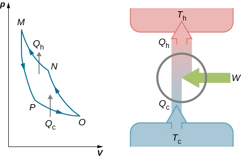
This work is equal to the area enclosed by the loop shown in the pV diagram of Figure 2. Because the initial and final states of the system are the same, the change of the internal energy of the gas in the cycle must be zero, that is, ΔEint=0. The first law of thermodynamics then gives W=Q−ΔEint=(Qh−Qc)−0, and W=Qh−Qc.
To find the efficiency of this engine, we first divide Qc by Qh:
QcQh=TcThlnVO/VPlnVN/VM.
When the adiabatic constant from step 2 is divided by that of step 4, we find
VOVP=VNVM.
Substituting this into the equation for Qc/Qh, we obtain
QcQh=TcTh.
Finally, with Equation 4.3.6, we find that the efficiency of this ideal gas Carnot engine is given by
e=1−TcTh.
An engine does not necessarily have to follow a Carnot engine cycle. All engines, however, have the same net effect, namely the absorption of heat from a hot reservoir, the production of work, and the discarding of heat to a cold reservoir. This leads us to ask: Do all reversible cycles operating between the same two reservoirs have the same efficiency? The answer to this question comes from the second law of thermodynamics discussed earlier: All reversible engine cycles produce exactly the same efficiency. Also, as you might expect, all real engines operating between two reservoirs are less efficient than reversible engines operating between the same two reservoirs. This too is a consequence of the second law of thermodynamics shown earlier.
The cycle of an ideal gas Carnot refrigerator is represented by the pV diagram of Figure 3. It is a Carnot engine operating in reverse. The refrigerator extracts heat Qc from a cold-temperature reservoir at Tc when the ideal gas expands isothermally. The gas is then compressed adiabatically until its temperature reaches Th, after which an isothermal compression of the gas results in heat Qh being discarded to a high-temperature reservoir at Th. Finally, the cycle is completed by an adiabatic expansion of the gas, causing its temperature to drop to Tc.

The work done on the ideal gas is equal to the area enclosed by the path of the pV diagram. From the first law, this work is given by
W=Qh−Qc.
An analysis just like the analysis done for the Carnot engine gives
QcTc=QhTh.
When combined with Equation 4.4.1, this yields
KR=TcTh−Tc
for the coefficient of performance of the ideal-gas Carnot refrigerator. Similarly, we can work out the coefficient of performance for a Carnot heat pump as
KP=QhQh−Qc=ThTh−Tc.
We have just found equations representing the efficiency of a Carnot engine and the coefficient of performance of a Carnot refrigerator or a Carnot heat pump, assuming an ideal gas for the working substance in both devices. However, these equations are more general than their derivations imply. We will soon show that they are both valid no matter what the working substance is.
Carnot summarized his study of the Carnot engine and Carnot cycle into what is now known as Carnot’s principle:
Carnot’s Principle
No engine working between two reservoirs at constant temperatures can have a greater efficiency than a reversible engine.
This principle can be viewed as another statement of the second law of thermodynamics and can be shown to be equivalent to the Kelvin statement and the Clausius statement.
Example 1: The Carnot Engine
A Carnot engine has an efficiency of 0.60 and the temperature of its cold reservoir is 300 K. (a) What is the temperature of the hot reservoir? (b) If the engine does 300 J of work per cycle, how much heat is removed from the high-temperature reservoir per cycle? (c) How much heat is exhausted to the low-temperature reservoir per cycle?
Strategy
From the temperature dependence of the thermal efficiency of the Carnot engine, we can find the temperature of the hot reservoir. Then, from the definition of the efficiency, we can find the heat removed when the work done by the engine is given. Finally, energy conservation will lead to how much heat must be dumped to the cold reservoir.
Solution
- From e=1−Tc/Th we have 0.60=1−300KTh, so that the temperature of the hot reservoir is Th=300K1−0.60=750K.
- By definition, the efficiency of the engine is e=W/Q, so that the heat removed from the high-temperature reservoir per cycle is Qh=We=300J0.60=500J.
- From the first law, the heat exhausted to the low-temperature reservoir per cycle by the engine is Qc=Qh−W=500J−300J=200J.
Significance
A Carnot engine has the maximum possible efficiency of converting heat into work between two reservoirs, but this does not necessarily mean it is 100% efficient. As the difference in temperatures of the hot and cold reservoir increases, the efficiency of a Carnot engine increases.
Example 2: A Carnot Heat Pump
Imagine a Carnot heat pump operates between an outside temperature of 0oC and an inside temperature of 20.0oC. What is the work needed if the heat delivered to the inside of the house is 30.0 kJ?
Strategy
Because the heat pump is assumed to be a Carnot pump, its performance coefficient is given by KP=Qh/W=Th/(Th−Tc). Thus, we can find the work W from the heat delivered Qh.
Solution
The work needed is obtained from
W=Qh/KP=Qh(Th−Tc)/Th=30kJ×(293K−273K)/293K=2kJ.
Significance
We note that this work depends not only on the heat delivered to the house but also on the temperatures outside and inside. The dependence on the temperature outside makes them impractical to use in areas where the temperature is much colder outside than room temperature.
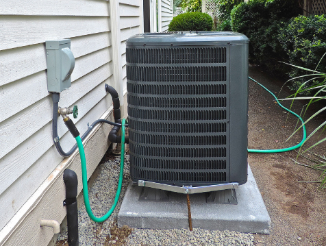
In terms of energy costs, the heat pump is a very economical means for heating buildings (Figure 4). Contrast this method with turning electrical energy directly into heat with resistive heating elements. In this case, one unit of electrical energy furnishes at most only one unit of heat. Unfortunately, heat pumps have problems that do limit their usefullness. They are quite expensive to purchase compared to resistive heating elements, and, as the performance coefficient for a Carnot heat pump shows, they become less effective as the outside temperature decreases. In fact, below about −10oC, the heat they furnish is less than the energy used to operate them.

Exercise 1
A Carnot engine operates between reservoirs at 400oC and 30oC.
- What is the efficiency of the engine?
- If the engine does 5.0 J of work per cycle, how much heat per cycle does it absorb from the high-temperature reservoir?
- How much heat per cycle does it exhaust to the cold-temperature reservoir?
- What temperatures at the cold reservoir would give the minimum and maximum efficiency?
- Answer a
-
e=1−Tc/Th=0.55
- Answer b
-
Qh=eW=9.1J
- Answer c
-
Qc=Qh−W=4.1J
- Answer d
-
−273oC and 400oC
Exercise 2
A Carnot refrigerator operates between two heat reservoirs whose temperatures are 0oC and 25oC.
- What is the coefficient of performance of the refrigerator?
- If 200 J of work are done on the working substance per cycle, how much heat per cycle is extracted from the cold reservoir?
- How much heat per cycle is discarded to the hot reservoir?
- Answer a
-
KR=Tc/(Th−Tc)=10.9
- Answer b
-
Qc=KRW=2.18kJ
- Answer c
-
Qh=Qc+W=2.38kJ


