2.6: Electric Field Diagrams

Learning Objectives

By the end of this section, you will be able to:

• Explain the purpose of an electric field diagram
• Describe the relationship between a vector diagram and a field line diagram
• Explain the rules for creating a field diagram and why these rules make physical sense
• Sketch the field of an arbitrary source charge

Now that we have experience calculating electric fields, let’s try to gain some insight into their geometry. As mentioned earlier, our model is that the charge on an object (the source charge) alters space in the region around it in such a way that when another charged object (the test charge) is placed in that region of space, that test charge experiences an electric force. The concepts of electric field vectors and field lines and their corresponding diagrams enable us to visualize how the space is altered, allowing us to visualize the field. The purpose of this section is to enable you to create sketches of this geometry, so we will list the specific steps and rules involved in creating an accurate and useful sketch of an electric field.

It is important to remember that electric fields are three-dimensional. Although we include some pseudo-three-dimensional images in this book, several diagrams (both here and in subsequent chapters) will be two-dimensional projections or cross-sections. Always keep in mind that, in fact, you are looking at a three-dimensional phenomenon.

Field-Vector Diagrams

Our starting point is the physical fact that the electric field of the source charge causes a test charge in that field to experience a force. By definition, electric field vectors point in the same direction as the electric force that a (hypothetical) positive test charge would experience if placed in the field (Figure \(\PageIndex{1}\)). This kind of diagram is called a electric field-vector diagram.

Figure \(\PageIndex{1}\): Electric field vector diagrams of a positive point charge. A large number of field vectors are shown. Like all vector arrows, the length of each vector is proportional to the magnitude of the field at each point. (a) Field in two dimensions; (b) field in three dimensions.

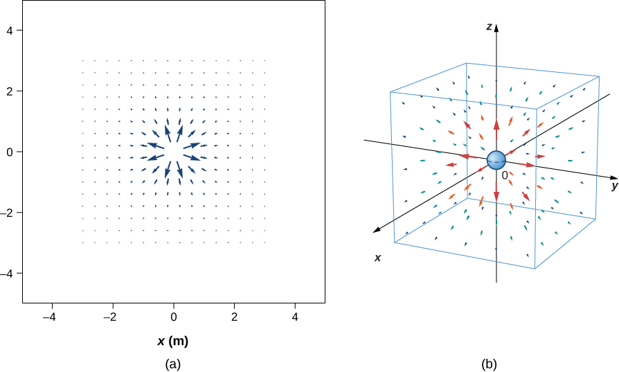
We plotted many field vectors in the figure using a uniform distribution of points around the source charge. Because the electric field is a vector, the arrows that we draw correspond at every point in space to both the magnitude and the direction of the field at that point. As always, the length of the arrow that we draw corresponds to the magnitude of the field vector at that point. For a point source charge, the length decreases by the square of the distance from the source charge. In addition, the direction of the field vector is radially away from the source charge because a positive test charge would experience a force in that direction in that field. (Again, remember that the actual field is three-dimensional; there are also field lines pointing out of and into the page.)

Finally, it should be noted that the field vectors in these diagrams should not be interpreted to have any spatial extent. In other words, the electric field vector acts only on a test charge placed at its starting point and not other points along the extent of the vector. Neighboring points can have vectors pointing in different directions, and if the density of points is high enough or the field vectors are long enough, the vectors may cross. These cases have no ambiguity or problem because the resulting field vectors are interpreted as acting at different points in space.

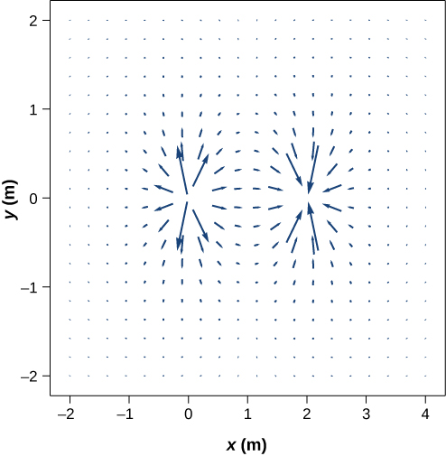
Field-vector diagrams can sometimes become less useful as the source charge distribution becomes more complicated. For example, consider the vector field diagram of a dipole (Figure \(\PageIndex{2}\)).

Figure \(\PageIndex{2}\): The vector field diagram of a dipole. Even with just two identical charges, the vector field diagram becomes difficult to understand.

Field-Line Diagrams

There is a more useful way to present the same information. Rather than drawing a large number of increasingly smaller vector arrows, we connect them all together, forming continuous lines and curves, as shown in Figure \(\PageIndex{3}\). This style of visualization is called a field-line diagram.

Figure \(\PageIndex{3}\): (a) The electric field line diagram of a positive point charge. (b) The field line diagram of a dipole. In both diagrams, the magnitude of the field is indicated by the field line density. The field vectors (not shown here) are everywhere tangent to the field lines.

Although it may not be obvious initially, these field-line diagrams convey the same information about the electric field as the field-vector diagrams. First, the direction of the field at every point is simply the direction of the field vector at that same point. In other words, at any point in space, the field vector at each point is tangent to the field line at that same point. The arrowhead placed on a field line indicates its direction.

But how is the magnitude of the field indicated since we no longer have the length of a vector to show us? The magnitude is instead indicated by the field-line density—that is, the number of field lines per unit area passing through a small cross-sectional area perpendicular to the electric field. This field-line density is drawn to be proportional to the magnitude of the field at that cross-section. As a result, if the field lines are close together (that is, the field line density is greater), the field's magnitude is large in that region. If the field lines are far apart at the cross-section, this indicates the field's magnitude is small. Figure \(\PageIndex{4}\) shows the idea.

Figure \(\PageIndex{4}\): Electric field lines passing through imaginary areas. Since the number of lines passing through each area is the same, but the areas themselves are different, the field line density is different. This indicates different magnitudes of the electric field at these points.

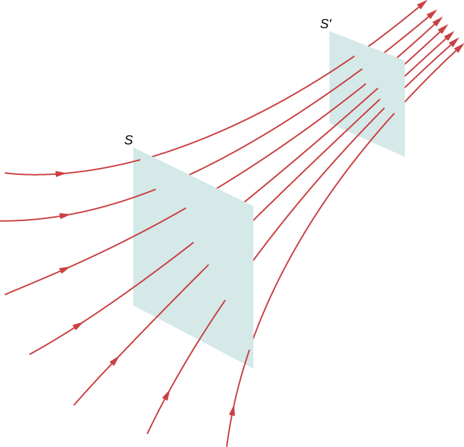
In Figure \(\PageIndex{4}\), the same number of field lines passes through both surfaces \(S\) and \(S'\), but the surface \(S\) is larger than surface \(S'\). Therefore, the density of field lines (number of lines per unit area) is larger at the location of \(S'\), indicating that the electric field is stronger at the location of \(S'\) than at \(S\). The rules for creating an electric field diagram are as follows.

Problem-Solving Strategy: Drawing Electric Field Lines

1. Electric field lines either originate on positive charges or come in from infinity and either terminate on negative charges or extend out to infinity.
2. The number of field lines originating or terminating at a charge is proportional to the magnitude of that charge. A charge of 2\(q\) will have twice as many lines as a charge of \(q\).
3. At every point in space, the field vector at that point is tangent to the field line at that same point.
4. The field line density at any point in space is proportional to (and therefore is representative of) the magnitude of the field at that point in space.
5. Field lines can never cross. Since a field line represents the direction of the field at a given point, if two field lines crossed at some point, that would imply that the electric field was pointing in two different directions at a single point. This result would suggest that the (net) force on a test charge placed at that point would point in two different directions. Since this situation is obviously impossible, field lines must never cross.

Always keep in mind that field lines serve only as a convenient way to visualize the electric field; they are not physical entities. Although the direction and relative intensity of the electric field can be deduced from a set of field lines, the lines can also be misleading. For example, the field lines drawn to represent the electric field in a region must, by necessity, be discrete. However, the actual electric field in that region exists at every point in space.

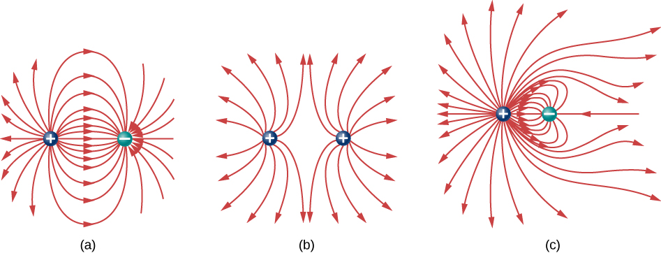
Field lines for three groups of discrete charges are shown in Figure \(\PageIndex{5}\). Since the charges in parts (a) and (b) have the same magnitude, the same number of field lines are shown starting from or terminating on each charge. In (c), however, we draw three times as many field lines leaving the \(+3q\) charge as entering the \(-q\). The field lines that do not terminate at \(-q\) emanate outward from the charge configuration to infinity.

Figure \(\PageIndex{5}\): Three typical electric field diagrams. (a) A dipole. (b) Two identical charges. (c) Two charges with opposite signs and different magnitudes. Can you tell from the diagram which charge has the larger magnitude?

The ability to construct an accurate electric field diagram is an important, useful skill; it makes it much easier to estimate, predict, and calculate the electric field of a source charge. The best way to develop this skill is with software that allows you to place source charges and then draw the net field upon request. One such simulation is given below. Practice drawing field diagrams on your own, and then check your predictions with the computer-drawn diagrams.

PhET Simulation: Charges and Fields

Instructions:

1. Make sure that the "Electric Field," "Values," and "Grid" boxes are checked in the box in the upper right corner of the screen.
2. Add one positive 1 nC charge to the center of the main window by dragging and dropping it from the box at the bottom of the window.
3. Observe the resulting electric field. By default, all the arrows will be the same length, and the field's strength will be designated by the arrow's brightness (i.e., dimmer arrows are weaker field strengths).
4. Add a sensor to the window by dragging and dropping it from the box at the bottom. Move the sensor around and observe how the magnitude and direction of the net field change. (Note that the electric field is given in units of V/m, where 1 V/m = 1 N/C).
5. Add a second positive charge to the window. Arrange the two charges in a horizontal line along the midline of the window, like in part (a) of Exercise \(\PageIndex{1B}\) of the previous section. Move the sensor around the window and observe how the magnitude and direction of the field changes. Does superposition hold? Do you see the same qualitative result as in the exercise?
6. Replace the left positive charge with a negative charge, like in part (b) of Exercise \(\PageIndex{1B}\) in the previous section. Does superposition hold? Do you see the same qualitative result as in the exercise?
7. Experiment with other combinations of three or more positive and negative charges, and observe how the electric field changes. Does the field pattern make sense based on superposition?

Source: Charges and Fields

Simulation by PhET Interactive Simulations, University of Colorado Boulder, licensed under CC-BY-4.0 (opens in new window).