2.7: Common Models of Electric Field

LEARNING OBJECTIVES

By the end of this section, you will be able to:

• Explain the concept of continuous charge distribution and explain why it is used.
• List and apply electric field models for some common geometric distributions of charge.
• Evaluate limiting cases of electric field models.

Continuous Charge Distributions

The charge distributions we have seen so far have been composed of discrete charges, in other words, made up of individual point particles. However, in many practical situations, there are so many charges in the system (often \(10^{22}\) or more!) that it is not possible to use superposition to calculate the electric field from each charge individual. To deal with this situation, we will introduce the approximation of a continuous charge distribution with at least one nonzero dimension. If a charge distribution is continuous rather than discrete, we can generalize the definition of the electric field. We divide the charge into infinitesimal pieces and treat each as a point charge. When we used superposition to calculate the total electric field at a test location using a continuous distribution, the discrete sum of electric-field contributions from discrete charges turns into an integral of electric-field contributions over all the infinitesimal "bits" of charge in the system.

Note that because charge is actually quantized, there is no such thing as a “truly” continuous charge distribution. However, in most practical cases, the total charge creating the field involves such a huge number of discrete charges that we can safely ignore the discrete nature of the charge and consider it to be continuous. This is exactly the kind of approximation we make when we model a bucket of water as a continuous fluid, rather than a collection of individual \(\ce{H2O}\) molecules.

When we use the assumption of continuous distribution of charge, the mathematics of calculating the electric field can still be challenging. In some special cases, we can construct the integrals, perform the integration analytically, and then write down closed-form formulas for the electric field at test locations in space. However, in general, it is often necessary to use computer simulations to calculate the electric field throughout the space surrounding the charge distribution.

In this chapter, we will summarize several models corresponding to the most common geometric distributions of charge. In each of these models, the electric field can be written in a closed-form expression for a specified region of space around the charge distribution. Students who are interested in the details of the calculations should refer to the section on Electric Fields of Charge Distributions in the chapter on Direct Calculation of Electrical Quantities from Charge Distributions. We will make use of these results in later chapters.

Electric Fields of Common Charge Distributions

In the following results, it is assumed that the charge density is uniform on the object or, in other words, the charge per unit length or charge per area is the same everywhere on the object.

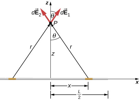
Finite Line Segment of Charge

Suppose a finite line segment of charge is located along the x-axis, as illustrated in Fig. \(\PageIndex{1}\). Assume that the segment has charge density \(\lambda\) (e.g., in coulombs per meters). The electric field along the perpendicular bisector of the segment at a distance z away from the segment is

\[\vec{E}(z) = \dfrac{1}{4 \pi \epsilon_0} \dfrac{\lambda L}{z\sqrt{z^2 + \dfrac{L^2}{4}}} \, \hat{k}. \ \ \ \ \text{(finite line segment)} \label{finitesegment}\]

Observe that if the charge density \(\lambda\) is positive, then the electric field points away from the segment. Otherwise, if the charge density \(\lambda\) is negative, then the electric field points toward the segment.

Figure \(\PageIndex{1}\): A uniformly charged segment of wire and its coordinate system. The electric field at point \(P\) can be found by applying the superposition principle to symmetrically placed charge elements and then integrating.

Infinite Line of Charge

If the length of the finite segment is allowed to go to infinite in both directions, then Equation \ref{finitesegment} becomes

\[\vec{E}(z) = \dfrac{1}{4 \pi \epsilon_0} \dfrac{2\lambda}{z}\hat{k} = \dfrac{\lambda}{2 \pi \epsilon_0 z}\hat{k}. \ \ \ \ \text{(infinite line)}\label{infiniteline}\]

In contrast to a point charge which falls off as the inverse square of the distance from the charge (\(1/r^2\)), the electric field of an infinite line charge falls off as the simple reciprocal of the distance from the line (\(1/z\)). Of course, no actual infinite line charges exist, so what is the purpose of this result? The answer is that if a line charge is sufficiently long as compared to the separation distance of the test location, then Equation \ref{infiniteline} will be a good approximation and certainly simpler than the exact result of Equation \ref{finitesegment}.

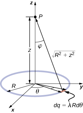
Ring of Charge

If we take a finite line segment with linear charge density \(\lambda\) and total charge \( q_0 \) and wrap it into a closed circular loop, then we get a ring of charge of radius \( R \) (Fig. \(\PageIndex{2}\)). The electric field at a distance \( z \) from the plane of the ring along its symmetry axis is

\[ \vec{E}(z) = \dfrac{1}{4\pi \epsilon_0} \dfrac{2\pi \lambda Rz}{(z^2 + R^2)^{3/2}} \hat{k} =
\dfrac{1}{4\pi \epsilon_0} \dfrac{q_{tot}z}{(z^2 + R^2)^{3/2}} \hat{k}. \ \ \ \ \text{(ring)} \label{ring}\]

Figure \(\PageIndex{2}\): A ring of charge of radius \( R \) and its coordinate system. The electric field at point \(P\) can be found by applying the superposition principle to symmetrically placed charge elements and integrating.

Exercise \(\PageIndex{1}\)

What is the electric field along the axis of the ring in the limit that \(z \gg R\)?

Answer

\[\vec{E} \approx \dfrac{1}{4\pi \epsilon_0} \dfrac{q_{tot}}{z^2} \hat{z}, \nonumber \]

which is the expression for the field of a point charge \(q_{tot}\). (If you get far enough away from a ring, it looks pointlike!)

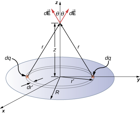
Disk of Charge

Once we know the electric field along the axis of a ring of charge, we can use this result to find the electric field along the axis of a disk of charge because a disk of charge can be modeled as a set of rings of charge of increasing radius (Fig. \(\PageIndex{3}\). The electric field for a disk of radius \(R\) and uniform surface charge density \(\sigma\) (coulombs per m\(^2\)) along the axis of the disk at a distance \(z\) from the disk is

\[\vec{E}(z) = \dfrac{1}{4 \pi \epsilon_0} \left( 2 \pi \sigma - \dfrac{2 \pi \sigma z}{\sqrt{z^2 + R^2}}\right)\hat{k}
=\dfrac{\sigma}{2 \epsilon_0} \left( 1 - \dfrac{z}{\sqrt{z^2 + R^2}}\right)\hat{k}. \ \ \ \ \text{(disk)}\label{disk}\]

Figure \(\PageIndex{4}\): A ring of charge of radius \( R \) and its coordinate system. The electric field at distance \(z\) can be found by applying the superposition principle to rings of increasing radius and integrating.

Exercise \(\PageIndex{2}\)

What is the electric field along the axis of the disk in the limit that \(z \gg R\)?

Answer

\[\vec{E}(z) \approx \dfrac{1}{4 \pi \epsilon_0} \dfrac{\sigma \pi R^2}{z^2} \hat{k},\nonumber\]

which is the expression for the field of a point charge \(Q = \sigma \pi R^2\). (If you get far enough away from a disk, it looks pointlike!)

Exercise \(\PageIndex{3}\)

How would the above limit change with a uniformly charged rectangle instead of a disk?

Answer

The result would be the same except that the point charge would be \(Q = \sigma ab\) where \(a\) and \(b\) are the sides of the rectangle.

Infinite Plane

As \(R \rightarrow \infty\), Equation \ref{disk} reduces to the field of an infinite plane, which is a flat sheet whose area is much, much greater than its thickness, and also much, much greater than the distance at which the field is to be calculated:

\[ \vec{E}(z) = \left\{ \begin{array}{ll}
\dfrac{\sigma}{2 \epsilon_0} \ \ \hat{k} & \mbox{if \(z > 0\)} \\
\dfrac{\sigma}{2 \epsilon_0} (-\hat{k}) & \mbox{if \(z < 0\)}
\end{array}
\right. \label{infiniteplane} \]

Note that this field is constant. This surprising result is, again, an artifact of our limit, although one that we will use repeatedly in the future. To understand why this happens, imagine being placed above an infinite plane of constant charge. Does the plane look any different if you vary your altitude? No—you still see the plane going off to infinity, no matter how far you are from it. The direction of the field below the plane is opposite to the direction above the plane because the field will always either point away from the plane (if positively charged) or toward the plane (if negatively charged).

Example \(\PageIndex{4}\): The Field of Two Infinite Planes

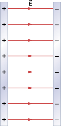
Find the electric field everywhere resulting from two infinite planes with equal but opposite charge densities (Figure \(\PageIndex{5}\)).

Figure \(\PageIndex{5}\): Two charged infinite planes. Note the direction of the electric field.

Strategy

We already know the electric field resulting from a single infinite plane, so we may use the principle of superposition to find the field from two.

Solution

The electric field points away from the positively charged plane and toward the negatively charged plane. Since the \(\sigma\) are equal and opposite, this means that in the region outside of the two planes, the electric fields cancel each other out to zero. However, in the region between the planes, the electric fields add, and we get

\[\vec{E} = \dfrac{\sigma}{\epsilon_0}\hat{i} \nonumber\]

for the electric field. The \(\hat{i}\) is because, in the figure, the field is pointing in the +x-direction.

Significance

Systems that may be approximated as two infinite planes provide a useful means of creating uniform electric fields. This approach can also be used to model a charged parallel-plate capacitor.

Exercise \(\PageIndex{4}\)

What would the electric field look like in a system with two parallel positively charged planes with equal charge densities?

Answer

The electric field would be zero in between the planes and have magnitude \(\dfrac{\sigma}{\epsilon_0}\) everywhere else.