Search

Text Color

Margin Size

Font Type

Enable Dyslexic Font

7.8: Application - RC Circuits with AC

Last updated

Nov 17, 2024
Save as PDF
- 7.7: Application - RC Circuits
- 7.9: Capacitance (Summary)

$\newcommand{\vecs}[1]{\overset { \scriptstyle \rightharpoonup} {\mathbf{#1}} }$

$\newcommand{\vecd}[1]{\overset{-\!-\!\rightharpoonup}{\vphantom{a}\smash {#1}}}$

$\newcommand{\id}{\mathrm{id}}$ $\newcommand{\Span}{\mathrm{span}}$

( \newcommand{\kernel}{\mathrm{null}\,}\) $\newcommand{\range}{\mathrm{range}\,}$

$\newcommand{\RealPart}{\mathrm{Re}}$ $\newcommand{\ImaginaryPart}{\mathrm{Im}}$

$\newcommand{\Argument}{\mathrm{Arg}}$ $\newcommand{\norm}[1]{\| #1 \|}$

$\newcommand{\inner}[2]{\langle #1, #2 \rangle}$

$\newcommand{\Span}{\mathrm{span}}$

$\newcommand{\id}{\mathrm{id}}$

$\newcommand{\Span}{\mathrm{span}}$

$\newcommand{\kernel}{\mathrm{null}\,}$

$\newcommand{\range}{\mathrm{range}\,}$

$\newcommand{\RealPart}{\mathrm{Re}}$

$\newcommand{\ImaginaryPart}{\mathrm{Im}}$

$\newcommand{\Argument}{\mathrm{Arg}}$

$\newcommand{\norm}[1]{\| #1 \|}$

$\newcommand{\inner}[2]{\langle #1, #2 \rangle}$

$\newcommand{\Span}{\mathrm{span}}$ $\newcommand{\AA}{\unicode[.8,0]{x212B}}$

$\newcommand{\vectorA}[1]{\vec{#1}} % arrow$

$\newcommand{\vectorAt}[1]{\vec{\text{#1}}} % arrow$

$\newcommand{\vectorB}[1]{\overset { \scriptstyle \rightharpoonup} {\mathbf{#1}} }$

$\newcommand{\vectorC}[1]{\textbf{#1}}$

$\newcommand{\vectorD}[1]{\overrightarrow{#1}}$

$\newcommand{\vectorDt}[1]{\overrightarrow{\text{#1}}}$

$\newcommand{\vectE}[1]{\overset{-\!-\!\rightharpoonup}{\vphantom{a}\smash{\mathbf {#1}}}}$

$\newcommand{\vecs}[1]{\overset { \scriptstyle \rightharpoonup} {\mathbf{#1}} }$

$\newcommand{\vecd}[1]{\overset{-\!-\!\rightharpoonup}{\vphantom{a}\smash {#1}}}$

$\newcommand{\avec}{\mathbf a}$

$\newcommand{\bvec}{\mathbf b}$

$\newcommand{\cvec}{\mathbf c}$

$\newcommand{\dvec}{\mathbf d}$

$\newcommand{\dtil}{\widetilde{\mathbf d}}$

$\newcommand{\evec}{\mathbf e}$

$\newcommand{\fvec}{\mathbf f}$

$\newcommand{\nvec}{\mathbf n}$

$\newcommand{\pvec}{\mathbf p}$

$\newcommand{\qvec}{\mathbf q}$

$\newcommand{\svec}{\mathbf s}$

$\newcommand{\tvec}{\mathbf t}$

$\newcommand{\uvec}{\mathbf u}$

$\newcommand{\vvec}{\mathbf v}$

$\newcommand{\wvec}{\mathbf w}$

$\newcommand{\xvec}{\mathbf x}$

$\newcommand{\yvec}{\mathbf y}$

$\newcommand{\zvec}{\mathbf z}$

$\newcommand{\rvec}{\mathbf r}$

$\newcommand{\mvec}{\mathbf m}$

$\newcommand{\zerovec}{\mathbf 0}$

$\newcommand{\onevec}{\mathbf 1}$

$\newcommand{\real}{\mathbb R}$

$\newcommand{\twovec}[2]{\left[\begin{array}{r}#1 \\ #2 \end{array}\right]}$

$\newcommand{\ctwovec}[2]{\left[\begin{array}{c}#1 \\ #2 \end{array}\right]}$

$\newcommand{\threevec}[3]{\left[\begin{array}{r}#1 \\ #2 \\ #3 \end{array}\right]}$

$\newcommand{\cthreevec}[3]{\left[\begin{array}{c}#1 \\ #2 \\ #3 \end{array}\right]}$

$\newcommand{\fourvec}[4]{\left[\begin{array}{r}#1 \\ #2 \\ #3 \\ #4 \end{array}\right]}$

$\newcommand{\cfourvec}[4]{\left[\begin{array}{c}#1 \\ #2 \\ #3 \\ #4 \end{array}\right]}$

$\newcommand{\fivevec}[5]{\left[\begin{array}{r}#1 \\ #2 \\ #3 \\ #4 \\ #5 \\ \end{array}\right]}$

$\newcommand{\cfivevec}[5]{\left[\begin{array}{c}#1 \\ #2 \\ #3 \\ #4 \\ #5 \\ \end{array}\right]}$

$\newcommand{\mattwo}[4]{\left[\begin{array}{rr}#1 \amp #2 \\ #3 \amp #4 \\ \end{array}\right]}$

$\newcommand{\laspan}[1]{\text{Span}\{#1\}}$

$\newcommand{\bcal}{\cal B}$

$\newcommand{\ccal}{\cal C}$

$\newcommand{\scal}{\cal S}$

$\newcommand{\wcal}{\cal W}$

$\newcommand{\ecal}{\cal E}$

$\newcommand{\coords}[2]{\left\{#1\right\}_{#2}}$

$\newcommand{\gray}[1]{\color{gray}{#1}}$

$\newcommand{\lgray}[1]{\color{lightgray}{#1}}$

$\newcommand{\rank}{\operatorname{rank}}$

$\newcommand{\row}{\text{Row}}$

$\newcommand{\col}{\text{Col}}$

$\renewcommand{\row}{\text{Row}}$

$\newcommand{\nul}{\text{Nul}}$

$\newcommand{\var}{\text{Var}}$

$\newcommand{\corr}{\text{corr}}$

$\newcommand{\len}[1]{\left|#1\right|}$

$\newcommand{\bbar}{\overline{\bvec}}$

$\newcommand{\bhat}{\widehat{\bvec}}$

$\newcommand{\bperp}{\bvec^\perp}$

$\newcommand{\xhat}{\widehat{\xvec}}$

$\newcommand{\vhat}{\widehat{\vvec}}$

$\newcommand{\uhat}{\widehat{\uvec}}$

$\newcommand{\what}{\widehat{\wvec}}$

$\newcommand{\Sighat}{\widehat{\Sigma}}$

$\newcommand{\lt}{<}$

$\newcommand{\gt}{>}$

$\newcommand{\amp}{&}$

$\definecolor{fillinmathshade}{gray}{0.9}$

Learning Objectives

By the end of the section, you will be able to:

Interpret phasor diagrams and apply them to ac circuits with resistors and capacitors
Define the reactance for a resistor and capacitor to help understand how current in the circuit behaves compared to each of these devices

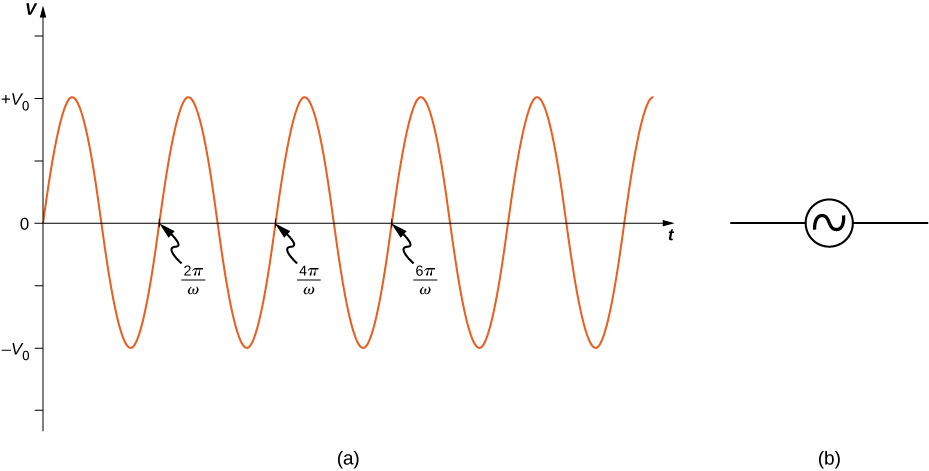
In this section, we study simple models of ac voltage sources connected to three circuit components: (1) a resistor and (2) a capacitor. The power furnished by an ac voltage source has an emf given by

$v(t) = V_0 \, sin \, \omega t,$

as shown in Figure $\PageIndex{1}$ . This sine function assumes we start recording the voltage when it is $v = 0 \, V$ at a time of $t = 0 \, s$ . A phase constant may be involved that shifts the function when we start measuring voltages, similar to the phase constant in the waves we studied in Waves. However, because we are free to choose when we start examining the voltage, we can ignore this phase constant for now. We can measure this voltage across the circuit components using one of two methods: (1) a quantitative approach based on our knowledge of circuits, or (2) a graphical approach that is explained in the coming sections.

Figure shows a sine wave with maximum and minimum values of the voltage being V0 and minus V0 respectively. Each positive slope of the wave, at the x-axis, marks one complete wavelength. These points are labeled in sequence: 2 pi by omega, 4 pi by omega and 6 pi by omega — Figure $\PageIndex{1}$ : (a) The output $v(t) = V_0 \, sin \, \omega t$ of an ac generator. (b) Symbol used to represent an ac voltage source in a circuit diagram.

Resistor

First, consider a resistor connected across an ac voltage source. From Kirchhoff’s loop rule, the instantaneous voltage across the resistor of Figure $\PageIndex{2a}$ is

$v_R(t) = V_0 \, sin \, \omega t$

and the instantaneous current through the resistor is

$i_R(t) = \frac{v_R(t)}{R} = \frac{V_0}{R} \, sin \, \omega t = I_0 \, sin \, \omega t.$

Figure a shows a circuit with an AC voltage source connected to a resistor. The source is labeled V0 sine omega t. Figure b shows sine waves of AC voltage and current on the same graph. Voltage has a greater amplitude than current and its maximum value is marked V0 on the y axis. The maximum value of current is marked I0. The voltage curve is labeled V subscript R parentheses t parentheses equal to V0 sine omega t. The current curve is labeled I subscript R parentheses t parentheses equal to I0 sine omega t. — Figure $\PageIndex{2}$ : (a) A resistor connected across an ac voltage source. (b) The current $i_R(t)$ through the resistor and the voltage $v_R(t)$ across the resistor. The two quantities are in phase.

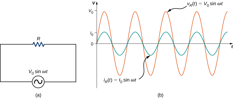
Here, $I_0 = V_0/R$ is the amplitude of the time-varying current. Plots of $i_R(t)$ and $v_R(t)$ are shown in Figure $\PageIndex{2b}$ . Both curves reach their maxima and minima at the same times, that is, the current through and the voltage across the resistor are in phase.

Graphical representations of the phase relationships between current and voltage are often useful in the analysis of ac circuits. Such representations are called phasor diagrams. The phasor diagram for $i_R(t)$ is shown in Figure $\PageIndex{3a}$ , with the current on the vertical axis. The arrow (or phasor) is rotating counterclockwise at a constant angular frequency $\omega$ , so we are viewing it at one instant in time. If the length of the arrow corresponds to the current amplitude $I_0$ , the projection of the rotating arrow onto the vertical axis is $i_R(t) = I_0 \, sin \, \omega t$ , which is the instantaneous current.

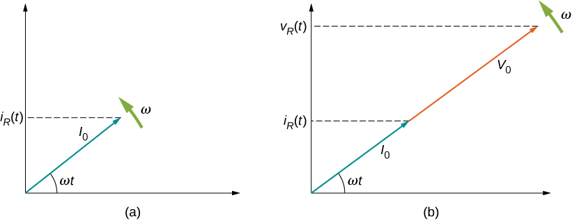
Figure shows the coordinate axes. An arrow labeled V0 starts from the origin and points up and right making an angle omega t with the x axis. An arrow labeled omega is shown near its tip, perpendicular to it, pointing up and left. The tip of the arrow V0 makes a y-intercept labeled V subscript C parentheses t parentheses. An arrow labeled I0 starts at the origin and points up and left. It is perpendicular to V0. It makes a y intercept labeled i subscript C parentheses t parentheses. A arrow labeled omega is shown near its tip, perpendicular to it, pointing down and left. — Figure $\PageIndex{3}$ : (a) The phasor diagram representing the current through the resistor of Figure $\PageIndex{2}$ (b) The phasor diagram representing both $i_R(t)$ and $v_R(t)$ .

The vertical axis on a phasor diagram could be either the voltage or the current, depending on the phasor that is being examined. In addition, several quantities can be depicted on the same phasor diagram. For example, both the current $i_R(t)$ and the voltage $v_R(t)$ are shown in the diagram of Figure $\PageIndex{3b}$ . Since they have the same frequency and are in phase, their phasors point in the same direction and rotate together. The relative lengths of the two phasors are arbitrary because they represent different quantities; however, the ratio of the lengths of the two phasors can be represented by the resistance, since one is a voltage phasor and the other is a current phasor.

Capacitor

Now let’s consider a capacitor connected across an ac voltage source. From Kirchhoff’s loop rule, the instantaneous voltage across the capacitor of Figure $\PageIndex{4a}$ is

$v_C(t) = V_0 \, sin \, \omega t.$

Recall that the charge in a capacitor is given by $Q = CV$ . This is true at any time measured in the ac cycle of voltage. Consequently, the instantaneous charge on the capacitor is

$q(t) = Cv_C(t) = CV_0 \, sin \, \omega t.$

Since the current in the circuit is the rate at which charge enters (or leaves) the capacitor,

$i_C(t) = \frac{dq(t)}{dt} = \omega CV_0 \, cos \, \omega t = I_0 \, cos \, \omega t,$

where $I_0 = \omega CV_0$ is the current amplitude. Using the trigonometric relationship $cos \, \omega t = sin (\omega t + \pi/2)$ , we may express the instantaneous current as

$i_C(t) = I_0 \, sin \left(\omega t + \frac{\pi}{2}\right).$

Dividing $V_0$ by $I_0$ , we obtain an equation that looks similar to Ohm’s law:

$\frac{V_0}{I_0} = \frac{1}{\omega C} = X_C. \label{15.3}$

The quantity $X_C$ is analogous to resistance in a dc circuit in the sense that both quantities are a ratio of a voltage to a current. As a result, they have the same unit, the ohm. Keep in mind, however, that a capacitor stores and discharges electric energy, whereas a resistor dissipates it. The quantity $X_C$ is known as the capacitive reactance of the capacitor, or the opposition of a capacitor to a change in current. It depends inversely on the frequency of the ac source—high frequency leads to low capacitive reactance.

Figure a shows a circuit with an AC voltage source connected to a capacitor. The source is labeled V0 sine omega t. Figure b shows sine waves of AC voltage and current on the same graph. Voltage has a greater amplitude than current and its maximum value is marked V0 on the y axis. The maximum value of current is marked I0. The two curves have the same wavelength but are out of phase by one quarter wavelength. The voltage curve is labeled V subscript C parentheses t parentheses equal to V0 sine omega t. The current curve is labeled I subscript C parentheses t parentheses equal to I0 sine parentheses omega t plus pi by 2 parentheses — Figure $\PageIndex{4}$ : (a) A capacitor connected across an ac generator. (b) The current $i_C(t)$ through the capacitor and the voltage $v_C(t)$ across the capacitor. Notice that $i_C(t)$ leads $v_C(t)$ by $\pi/2$ rad.

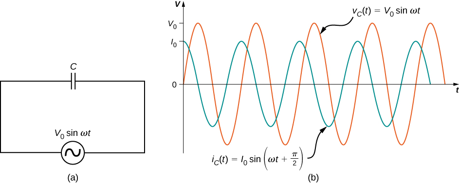
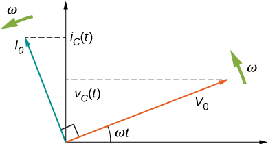
A comparison of the expressions for $v_C(t)$ and $i_C(t)$ shows that there is a phase difference of $\pi/2$ rad between them. When these two quantities are plotted together, the current peaks a quarter cycle (or $\pi/2$ rad) ahead of the voltage, as illustrated in Figure $\PageIndex{4b}$ . The current through a capacitor leads the voltage across a capacitor by $\pi/2$ rad, or a quarter of a cycle.

The corresponding phasor diagram is shown in Figure $\PageIndex{5}$ . Here, the relationship between $i_C(t)$ and $v_C(t)$ is represented by having their phasors rotate at the same angular frequency, with the current phasor leading by $\pi/2$ rad.

To this point, we have exclusively been using peak values of the current or voltage in our discussion, namely, $I_0$ and $V_0$ . However, if we average out the values of current or voltage, these values are zero. Therefore, we often use a second convention called the root mean square value, or rms value, in discussions of current and voltage. The rms operates in reverse of the terminology. First, you square the function, next, you take the mean, and then, you find the square root. As a result, the rms values of current and voltage are not zero. Appliances and devices are commonly quoted with rms values for their operations, rather than peak values. We indicate rms values with a subscript attached to a capital letter (such as $I_{rms}$ ).

Although a capacitor is basically an open circuit, an rms current, or the root mean square of the current, appears in a circuit with an ac voltage applied to a capacitor. Consider that

Note

$I_{rms} = \frac{I_0}{\sqrt{2}},$

where $I_0$ is the peak current in an ac system. The rms voltage, or the root mean square of the voltage, is

Note

$V_{rms} = \frac{V_0}{\sqrt{2}},$

where $V_0$ is the peak voltage in an ac system. The rms current appears because the voltage is continually reversing, charging, and discharging the capacitor. If the frequency goes to zero, which would be a dc voltage, $X_C$ tends to infinity, and the current is zero once the capacitor is charged. At very high frequencies, the capacitor’s reactance tends to zero—it has a negligible reactance and does not impede the current (it acts like a simple wire).

Contributors and Attributions

Samuel J. Ling (Truman State University), Jeff Sanny (Loyola Marymount University), and Bill Moebs with many contributing authors. This work is licensed by OpenStax University Physics under a Creative Commons Attribution License (by 4.0).

Learning Objectives

Resistor

Capacitor

Note

Note

Contributors and Attributions

Support Center

How can we help?