16.2: Electric Dipoles

Learning Objectives

By the end of this section, you will be able to:

• Define an electric dipole.
• Distinguish a permanent dipole from an induced dipole.
• Define and calculate an electric dipole moment.
• Explain the physical meaning of the dipole moment.
• Calculate the torque on a dipole in a uniform electric field.
• Define and calculate the electric potential of a dipole.

Earlier we discussed, and calculated, the electric field of a dipole: two equal and opposite charges that are “close” to each other. (In this context, “close” means that the distance \(d\) between the two charges is much, much less than the distance of the field point \(P\), the location where you are calculating the field.) Let’s now consider what happens to a dipole when it is placed in an external field \(\vec{E}\). We assume that the dipole is a permanent dipole; it exists without the field, and does not break apart in the external field.

Rotation of a Dipole due to an Electric Field

For now, we deal with only the simplest case: The external field is uniform in space. Suppose we have the situation depicted in Figure \(\PageIndex{1}\), where we denote the distance between the charges as the vector \(\vec{d}\), pointing from the negative charge to the positive charge.

Figure \(\PageIndex{1}\): A dipole in an external electric field. (a) The net force on the dipole is zero, but the net torque is not. As a result, the dipole rotates, becoming aligned with the external field. (b) The dipole moment is a convenient way to characterize this effect. The \(\vec{d}\) points in the same direction as \(\vec{p}\).

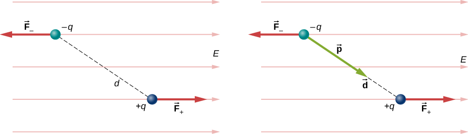
The forces on the two charges are equal and opposite, so there is no net force on the dipole. However, there is a torque:

\[\begin{align} \vec{r} &= \left(\dfrac{\vec{d}}{2} \times \vec{F}_+ \right) + \left(- \dfrac{\vec{d}}{2} \times \vec{F}_- \right) \\[4pt] &= \left[ \left(\dfrac{\vec{d}}{2}\right) \times \left(+q\vec{E}\right) + \left(-\dfrac{\vec{d}}{2}\right) \times \left(-q\vec{E}\right)\right] \\[4pt] &= q\vec{d} \times \vec{E}. \end{align}\]

The quantity \(qd\) (the magnitude of each charge multiplied by the vector distance between them) is a property of the dipole; its value, as you can see, determines the torque that the dipole experiences in the external field. It is useful, therefore, to define this product as the so-called dipole moment of the dipole:

\[\vec{p} \equiv q\vec{d}.\]

We can therefore write

\[\vec{\tau} = \vec{p} \times \vec{E}.\]

Recall that a torque changes the angular velocity of an object, the dipole, in this case. In this situation, the effect is to rotate the dipole (that is, align the direction of \(\vec{p}\)) so that it is parallel to the direction of the external field.

Induced Dipoles

Neutral atoms are, by definition, electrically neutral; they have equal amounts of positive and negative charge. Furthermore, since they are spherically symmetrical, they do not have a “built-in” dipole moment the way most asymmetrical molecules do. They obtain one, however, when placed in an external electric field, because the external field causes oppositely directed forces on the positive nucleus of the atom versus the negative electrons that surround the nucleus. The result is a new charge distribution of the atom, and therefore, an induced dipole moment (Figure \(\PageIndex{2}\)).

Figure \(\PageIndex{2}\): A dipole is induced in a neutral atom by an external electric field. The induced dipole moment is aligned with the external field.

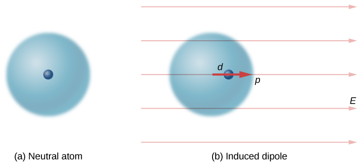
An important fact here is that, just as for a rotated polar molecule, the result is that the dipole moment ends up aligned parallel to the external electric field. Generally, the magnitude of an induced dipole is much smaller than that of an inherent dipole. For both kinds of dipoles, notice that once the alignment of the dipole (rotated or induced) is complete, the net effect is to decrease the total electric field

\[\vec{E}_{total} = \vec{E}_{external} + \vec{E}_{dipole}\]

in the regions outside the dipole charges (Figure \(\PageIndex{3}\)). By “outside” we mean further from the charges than they are from each other. This effect is crucial for capacitors, as you will see in Capacitance.

Figure \(\PageIndex{3}\): The net electric field is the vector sum of the field of the dipole plus the external field.

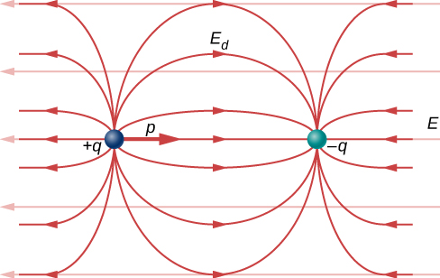
Recall that we found the electric field of a dipole. If we rewrite it in terms of the dipole moment we get:

\[\vec{E}(z) = \dfrac{1}{4 \pi \epsilon_0} \dfrac{\vec{p}}{z^3}.\]

The form of this field is shown in Figure \(\PageIndex{3}\). Notice that along the plane perpendicular to the axis of the dipole and midway between the charges, the direction of the electric field is opposite that of the dipole and gets weaker the further from the axis one goes. Similarly, on the axis of the dipole (but outside it), the field points in the same direction as the dipole, again getting weaker the further one gets from the charges.

Electric Potential of Dipole

An electric dipole is a system of two equal but opposite charges a fixed distance apart. This system is used to model many real-world systems, including atomic and molecular interactions. One of these systems is the water molecule, under certain circumstances. These circumstances are met inside a microwave oven, where electric fields with alternating directions make the water molecules change orientation. This vibration is the same as heat at the molecular level.

Example \(\PageIndex{3}\): Electric Potential of a Dipole

Consider the dipole in Figure \(\PageIndex{3}\) with the charge magnitude of \(q = 3.0 \, \mu \textrm{C}\) and separation distance \(d = 4.0 \, \textrm{cm}.\) What is the potential at the following locations in space? (a) (0, 0, 1.0 cm); (b) (0, 0, –5.0 cm); (c) (3.0 cm, 0, 2.0 cm).

Figure \(\PageIndex{3}\): A general diagram of an electric dipole, and the notation for the distances from the individual charges to a point \(\textrm{P}\) in space.

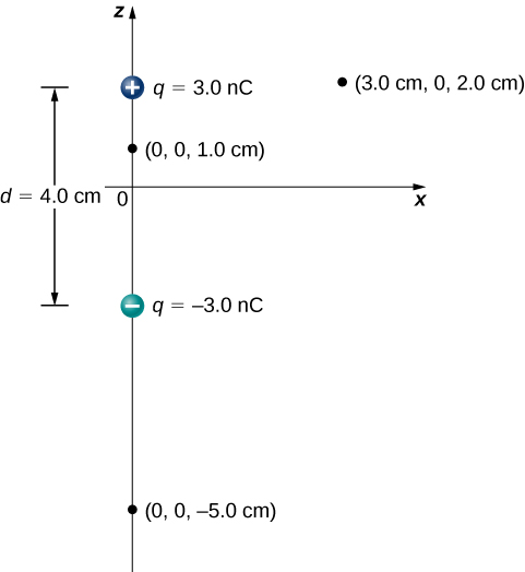
Strategy

Apply \(V_p = k \sum_1^N \dfrac{q_i}{r_i}\) to each of these three points.

Solution

a. \(V_p = k \sum_1^N \dfrac{q_i}{r_i} = (9.0 \times 10^9 \,\textrm{N} \cdot \textrm{m}^2/\textrm{C}^2) \left(\dfrac{3.0\space \textrm{nC}}{0.010 \, \textrm{m}} - \dfrac{3.0\space \textrm{nC}}{0.030 \, \textrm{m}}\right) = 1.8 \times 10^3 \, \textrm{V}\)

b. \(V_p = k \sum_1^N \dfrac{q_i}{r_i} = (9.0 \times 10^9 \, \textrm{N} \cdot \textrm{m}^2/\textrm{C}^2) \left(\dfrac{3.0\space \textrm{nC}}{0.070 \, \textrm{m}} - \dfrac{3.0\space \textrm{nC}}{0.030 \, \textrm{m}}\right) = -5.1 \times 10^2 \, \textrm{V}\)

c. \(V_p = k \sum_1^N \dfrac{q_i}{r_i} = (9.0 \times 10^9 \, \textrm{N} \cdot \textrm{m}^2/\textrm{C}^2) \left(\dfrac{3.0\space \textrm{nC}}{0.030 \, \textrm{m}} - \dfrac{3.0\space \textrm{nC}}{0.050 \, \textrm{m}}\right) = 3.6 \times 10^2 \, \textrm{V}\)

Significance

Note that evaluating potential is significantly simpler than electric field, due to potential being a scalar instead of a vector.

Exercise \(\PageIndex{1}\)

What is the potential on the \(x\)-axis? The \(z\)-axis?

Answer

The \(x\)-axis the potential is zero, due to the equal and opposite charges the same distance from it. On the \(z\)-axis, we may superimpose the two potentials; we will find that for \(z > > d\), again the potential goes to zero due to cancellation.

Now let us consider the special case when the distance of the point \(P\) from the dipole is much greater than the distance between the charges in the dipole, \(r >> d\); for example, when we are interested in the electric potential due to a polarized molecule such as a water molecule. This is not so far (infinity) that we can simply treat the potential as zero, but the distance is great enough that we can simplify our calculations relative to the previous example.

We start by noting that in Figure \(\PageIndex{4}\) the potential is given by

\[V_p = V_+ + V_- = k \left( \dfrac{q}{r_+} - \dfrac{q}{r_-} \right)\]

where

\[r_{\pm} = \sqrt{x^2 + \left(z \pm \dfrac{d}{2}\right)^2}.\]

Figure \(\PageIndex{4}\): A general diagram of an electric dipole, and the notation for the distances from the individual charges to a point \(P\) in space.

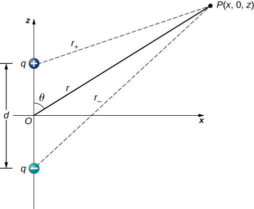
This is still the exact formula. To take advantage of the fact that \(r \gg d\), we rewrite the radii in terms of polar coordinates, with \(x = r \sin\theta\) and \(z = r \cos\theta\). This gives us

\[r_{\pm} = \sqrt{r^2 \sin^2 \theta + \left(r \cos\theta \pm \dfrac{d}{2} \right)^2}.\]

We can simplify this expression by pulling \(r\) out of the root,

\[r_{\pm} = \sqrt{\sin^2 \, \theta + \left(r \, \cos \, \theta \pm \dfrac{d}{2} \right)^2}\]

and then multiplying out the parentheses

\[r_{\pm} = r \sqrt{\sin^2\theta + \cos^2\theta \pm \cos\theta\, \dfrac{d}{r} + \left(\dfrac{d}{2r}\right)^2} = r\sqrt{1 \pm \cos\theta \, \dfrac{d}{r} + \left(\dfrac{d}{2r}\right)^2}.\]

The last term in the root is small enough to be negligible (remember \(r >> d\), and hence \((d/r)^2\) is extremely small, effectively zero to the level we will probably be measuring), leaving us with

\[r_{\pm} = r\sqrt{1 \pm \cos\theta \, \dfrac{d}{r}}.\]

Using the binomial approximation (a standard result from the mathematics of series, when \(a\) is small)

\[\dfrac{1}{\sqrt{1 \pm a}} \approx 1 \pm \dfrac{a}{2}\]

and substituting this into our formula for \(V_p\), we get

\[V_p = k\left[\dfrac{q}{r}\left(1 + \dfrac{d \cos\theta}{2r} \right) - \dfrac{q}{r}\left(1 - \dfrac{d \cos\theta}{2r}\right)\right] = k\dfrac{qd \cos\theta}{r^2}.\]

This may be written more conveniently if we define a new quantity, the electric dipole moment,

\[\vec{p} = q\vec{d},\]

where these vectors point from the negative to the positive charge. Note that this has magnitude \(qd\). This quantity allows us to write the potential at point \(P\) due to a dipole at the origin as

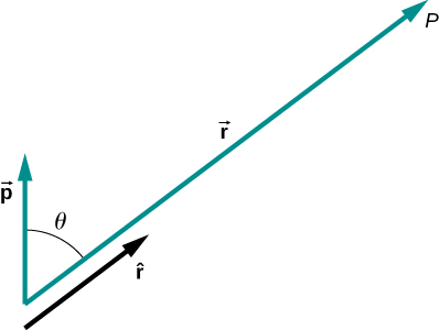
\[V_p = k\dfrac{\vec{p} \cdot \hat{r}}{r^2}.\]

A diagram of the application of this formula is shown in Figure \(\PageIndex{5}\).

Figure \(\PageIndex{5}\): The geometry for the application of the potential of a dipole.

There are also higher-order moments for quadrupoles, octupoles, and so on.