
3.6: Equipotential Surfaces and Conductors
- Page ID
- 32167

\( \newcommand{\vecs}[1]{\overset { \scriptstyle \rightharpoonup} {\mathbf{#1}} } \)
\( \newcommand{\vecd}[1]{\overset{-\!-\!\rightharpoonup}{\vphantom{a}\smash {#1}}} \)
\( \newcommand{\id}{\mathrm{id}}\) \( \newcommand{\Span}{\mathrm{span}}\)
( \newcommand{\kernel}{\mathrm{null}\,}\) \( \newcommand{\range}{\mathrm{range}\,}\)
\( \newcommand{\RealPart}{\mathrm{Re}}\) \( \newcommand{\ImaginaryPart}{\mathrm{Im}}\)
\( \newcommand{\Argument}{\mathrm{Arg}}\) \( \newcommand{\norm}[1]{\| #1 \|}\)
\( \newcommand{\inner}[2]{\langle #1, #2 \rangle}\)
\( \newcommand{\Span}{\mathrm{span}}\)
\( \newcommand{\id}{\mathrm{id}}\)
\( \newcommand{\Span}{\mathrm{span}}\)
\( \newcommand{\kernel}{\mathrm{null}\,}\)
\( \newcommand{\range}{\mathrm{range}\,}\)
\( \newcommand{\RealPart}{\mathrm{Re}}\)
\( \newcommand{\ImaginaryPart}{\mathrm{Im}}\)
\( \newcommand{\Argument}{\mathrm{Arg}}\)
\( \newcommand{\norm}[1]{\| #1 \|}\)
\( \newcommand{\inner}[2]{\langle #1, #2 \rangle}\)
\( \newcommand{\Span}{\mathrm{span}}\) \( \newcommand{\AA}{\unicode[.8,0]{x212B}}\)
\( \newcommand{\vectorA}[1]{\vec{#1}} % arrow\)
\( \newcommand{\vectorAt}[1]{\vec{\text{#1}}} % arrow\)
\( \newcommand{\vectorB}[1]{\overset { \scriptstyle \rightharpoonup} {\mathbf{#1}} } \)
\( \newcommand{\vectorC}[1]{\textbf{#1}} \)
\( \newcommand{\vectorD}[1]{\overrightarrow{#1}} \)
\( \newcommand{\vectorDt}[1]{\overrightarrow{\text{#1}}} \)
\( \newcommand{\vectE}[1]{\overset{-\!-\!\rightharpoonup}{\vphantom{a}\smash{\mathbf {#1}}}} \)
\( \newcommand{\vecs}[1]{\overset { \scriptstyle \rightharpoonup} {\mathbf{#1}} } \)
\( \newcommand{\vecd}[1]{\overset{-\!-\!\rightharpoonup}{\vphantom{a}\smash {#1}}} \)
\(\newcommand{\avec}{\mathbf a}\) \(\newcommand{\bvec}{\mathbf b}\) \(\newcommand{\cvec}{\mathbf c}\) \(\newcommand{\dvec}{\mathbf d}\) \(\newcommand{\dtil}{\widetilde{\mathbf d}}\) \(\newcommand{\evec}{\mathbf e}\) \(\newcommand{\fvec}{\mathbf f}\) \(\newcommand{\nvec}{\mathbf n}\) \(\newcommand{\pvec}{\mathbf p}\) \(\newcommand{\qvec}{\mathbf q}\) \(\newcommand{\svec}{\mathbf s}\) \(\newcommand{\tvec}{\mathbf t}\) \(\newcommand{\uvec}{\mathbf u}\) \(\newcommand{\vvec}{\mathbf v}\) \(\newcommand{\wvec}{\mathbf w}\) \(\newcommand{\xvec}{\mathbf x}\) \(\newcommand{\yvec}{\mathbf y}\) \(\newcommand{\zvec}{\mathbf z}\) \(\newcommand{\rvec}{\mathbf r}\) \(\newcommand{\mvec}{\mathbf m}\) \(\newcommand{\zerovec}{\mathbf 0}\) \(\newcommand{\onevec}{\mathbf 1}\) \(\newcommand{\real}{\mathbb R}\) \(\newcommand{\twovec}[2]{\left[\begin{array}{r}#1 \\ #2 \end{array}\right]}\) \(\newcommand{\ctwovec}[2]{\left[\begin{array}{c}#1 \\ #2 \end{array}\right]}\) \(\newcommand{\threevec}[3]{\left[\begin{array}{r}#1 \\ #2 \\ #3 \end{array}\right]}\) \(\newcommand{\cthreevec}[3]{\left[\begin{array}{c}#1 \\ #2 \\ #3 \end{array}\right]}\) \(\newcommand{\fourvec}[4]{\left[\begin{array}{r}#1 \\ #2 \\ #3 \\ #4 \end{array}\right]}\) \(\newcommand{\cfourvec}[4]{\left[\begin{array}{c}#1 \\ #2 \\ #3 \\ #4 \end{array}\right]}\) \(\newcommand{\fivevec}[5]{\left[\begin{array}{r}#1 \\ #2 \\ #3 \\ #4 \\ #5 \\ \end{array}\right]}\) \(\newcommand{\cfivevec}[5]{\left[\begin{array}{c}#1 \\ #2 \\ #3 \\ #4 \\ #5 \\ \end{array}\right]}\) \(\newcommand{\mattwo}[4]{\left[\begin{array}{rr}#1 \amp #2 \\ #3 \amp #4 \\ \end{array}\right]}\) \(\newcommand{\laspan}[1]{\text{Span}\{#1\}}\) \(\newcommand{\bcal}{\cal B}\) \(\newcommand{\ccal}{\cal C}\) \(\newcommand{\scal}{\cal S}\) \(\newcommand{\wcal}{\cal W}\) \(\newcommand{\ecal}{\cal E}\) \(\newcommand{\coords}[2]{\left\{#1\right\}_{#2}}\) \(\newcommand{\gray}[1]{\color{gray}{#1}}\) \(\newcommand{\lgray}[1]{\color{lightgray}{#1}}\) \(\newcommand{\rank}{\operatorname{rank}}\) \(\newcommand{\row}{\text{Row}}\) \(\newcommand{\col}{\text{Col}}\) \(\renewcommand{\row}{\text{Row}}\) \(\newcommand{\nul}{\text{Nul}}\) \(\newcommand{\var}{\text{Var}}\) \(\newcommand{\corr}{\text{corr}}\) \(\newcommand{\len}[1]{\left|#1\right|}\) \(\newcommand{\bbar}{\overline{\bvec}}\) \(\newcommand{\bhat}{\widehat{\bvec}}\) \(\newcommand{\bperp}{\bvec^\perp}\) \(\newcommand{\xhat}{\widehat{\xvec}}\) \(\newcommand{\vhat}{\widehat{\vvec}}\) \(\newcommand{\uhat}{\widehat{\uvec}}\) \(\newcommand{\what}{\widehat{\wvec}}\) \(\newcommand{\Sighat}{\widehat{\Sigma}}\) \(\newcommand{\lt}{<}\) \(\newcommand{\gt}{>}\) \(\newcommand{\amp}{&}\) \(\definecolor{fillinmathshade}{gray}{0.9}\)By the end of this section, you will be able to:
- Define equipotential surfaces and equipotential lines
- Explain the relationship between equipotential lines and electric field lines
- Map equipotential lines for one or two point charges
- Describe the potential of a conductor
- Compare and contrast equipotential lines and elevation lines on topographic maps
We can represent electric potentials (voltages) pictorially, just as we drew pictures to illustrate electric fields. This is not surprising, since the two concepts are related. Consider Figure \(\PageIndex{1}\), which shows an isolated positive point charge and its electric field lines, which radiate out from a positive charge and terminate on negative charges. We use blue arrows to represent the magnitude and direction of the electric field, and we use green lines to represent places where the electric potential is constant. These are called equipotential surfaces in three dimensions, or equipotential lines in two dimensions. The term equipotential is also used as a noun, referring to an equipotential line or surface. The potential for a point charge is the same anywhere on an imaginary sphere of radius r surrounding the charge. This is true because the potential for a point charge is given by \(V = kq/r\) and thus has the same value at any point that is a given distance r from the charge. An equipotential sphere is a circle in the two-dimensional view of Figure \(\PageIndex{1}\). Because the electric field lines point radially away from the charge, they are perpendicular to the equipotential lines.
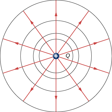
It is important to note that equipotential lines are always perpendicular to electric field lines. No work is required to move a charge along an equipotential, since \(\Delta V = 0\). Thus, the work is
\[W = - \Delta U = - q\Delta V = 0.\]
Work is zero if the direction of the force is perpendicular to the displacement. Force is in the same direction as \(E\), so motion along an equipotential must be perpendicular to \(E\). More precisely, work is related to the electric field by
\[\begin{align} W &= \vec{F} \cdot \vec{d} \label{eq5} \\[4pt] &= q\vec{E} \cdot \vec{d} \nonumber \\[4pt] &= qEd \, \cos \, \theta \nonumber \\[4pt] &= 0. \nonumber \end{align} \nonumber\]
Note that in Equation \ref{eq5}, \(E\) and \(F\) symbolize the magnitudes of the electric field and force, respectively. Neither \(q\) nor \(E\) is zero and \(d\) is also not zero. So \(\cos \, \theta\) must be 0, meaning \(\theta\) must be \(90^o\). In other words, motion along an equipotential is perpendicular to E.
One of the rules for static electric fields and conductors is that the electric field must be perpendicular to the surface of any conductor. This implies that a conductor is an equipotential surface in static situations. There can be no voltage difference across the surface of a conductor, or charges will flow. One of the uses of this fact is that a conductor can be fixed at what we consider zero volts by connecting it to the earth with a good conductor—a process called grounding. Grounding can be a useful safety tool. For example, grounding the metal case of an electrical appliance ensures that it is at zero volts relative to Earth.
Because a conductor is an equipotential, it can replace any equipotential surface. For example, in Figure \(\PageIndex{2}\), a charged spherical conductor can replace the point charge, and the electric field and potential surfaces outside of it will be unchanged, confirming the contention that a spherical charge distribution is equivalent to a point charge at its center.
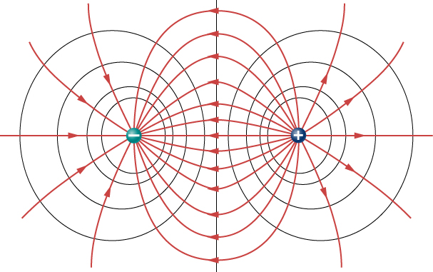
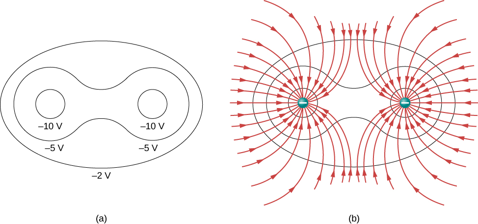
Figure \(\PageIndex{2}\) shows the electric field and equipotential lines for two equal and opposite charges. Given the electric field lines, the equipotential lines can be drawn simply by making them perpendicular to the electric field lines. Conversely, given the equipotential lines, as in Figure \(\PageIndex{2a}\), the electric field lines can be drawn by making them perpendicular to the equipotentials, as in Figure \(\PageIndex{2b}\).
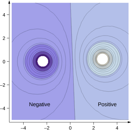
To improve your intuition, we show a three-dimensional variant of the potential in a system with two opposing charges. Figure \(\PageIndex{4}\) displays a three-dimensional map of electric potential, where lines on the map are for equipotential surfaces. The hill is at the positive charge, and the trough is at the negative charge. The potential is zero far away from the charges. Note that the cut off at a particular potential implies that the charges are on conducting spheres with a finite radius.
Figure \(\PageIndex{4}\): Electric potential map of two opposite charges of equal magnitude on conducting spheres. The potential is negative near the negative charge and positive near the positive charge. This dynamic image is powered by CalcPlot3D and can be viewed here.
A two-dimensional map of the cross-sectional plane that contains both charges is shown in Figure \(\PageIndex{5}\). The line that is equidistant from the two opposite charges corresponds to zero potential, since at the points on the line, the positive potential from the positive charge cancels the negative potential from the negative charge. Equipotential lines in the cross-sectional plane are closed loops, which are not necessarily circles, since at each point, the net potential is the sum of the potentials from each charge.
View this simulation to observe and modify the equipotential surfaces and electric fields for many standard charge configurations. There’s a lot to explore.
One of the most important cases is that of the familiar parallel conducting plates shown in Figure \(\PageIndex{6}\). Between the plates, the equipotentials are evenly spaced and parallel. The same field could be maintained by placing conducting plates at the equipotential lines at the potentials shown.
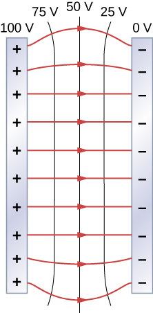
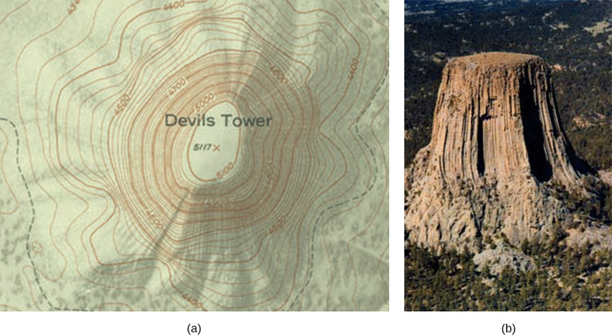
Consider the parallel plates Figure \(\PageIndex{6}\). These have equipotential lines that are parallel to the plates in the space between and evenly spaced. An example of this (with sample values) is given in Figure \(\PageIndex{6}\). We could draw a similar set of equipotential isolines for gravity on hills . If the hill has any extent at the same slope, the isolines along that extent would be parallel to each other. Furthermore, in regions of constant slope, the isolines would be evenly spaced. An example of real topographic lines is shown in Figure \(\PageIndex{7}\).
Example \(\PageIndex{1}\): Calculating Equipotential Lines
You have seen the equipotential lines of a point charge in Figure \(\PageIndex{1}\). How do we calculate them? For example, if we have a \(+10-nC\) charge at the origin, what are the equipotential surfaces at which the potential is (a) 100 V, (b) 50 V, (c) 20 V, and (d) 10 V?
Strategy
Set the equation for the potential of a point charge equal to a constant and solve for the remaining variable(s). Then calculate values as needed.
Solution
In \(V = k\dfrac{q}{r}\), let V be a constant. The only remaining variable is r; hence, \(r = k\dfrac{q}{V} = constant\). Thus, the equipotential surfaces are spheres about the origin. Their locations are:
- \(r = k\dfrac{q}{V} = \left(8.99 \times 10^9 \, Nm^2/C^2\right) \dfrac{(10 \times 10^{-9} C)}{100 \, V} = 0.90 \, m\);
- \(r = k\dfrac{q}{V} = \left(8.99 \times 10^9 \, Nm^2/C^2\right) \dfrac{(10 \times 10^{-9} C)}{50 \, V} = 1.8 \, m\);
- \(r = k\dfrac{q}{V} = \left(8.99 \times 10^9 \, Nm^2/C^2\right) \dfrac{(10 \times 10^{-9} C)}{20 \, V} = 4.5 \, m\);
- \(r = k\dfrac{q}{V} = \left(8.99 \times 10^9 \, Nm^2/C^2\right) \dfrac{(10 \times 10^{-9} C)}{10 \, V} = 9.0 \, m\).
Significance
This means that equipotential surfaces around a point charge are spheres of constant radius, as shown earlier, with well-defined locations.
Example \(\PageIndex{2}\): Potential Difference between Oppositely Charged Parallel Plates
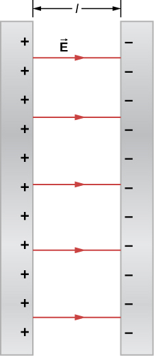
Two large conducting plates carry equal and opposite charges, with a surface charge density \(\sigma\) of magnitude \(6.81 \times 10^{-7} C/m\), as shown in Figure \(\PageIndex{8}\). The separation between the plates is \(l = 6.50 \, mm\).
- What is the electric field between the plates?
- What is the potential difference between the plates?
- What is the distance between equipotential planes which differ by 100 V?
Strategy
- Since the plates are described as “large” and the distance between them is not, we will approximate each of them as an infinite plane, and apply the result from Gauss’s law in the previous chapter.
- Use \(\Delta V_{AB} = - \int_A^B \vec{E} \cdot d\vec{l}\).
- Since the electric field is constant, find the ratio of 100 V to the total potential difference; then calculate this fraction of the distance.
Solution
a. The electric field is directed from the positive to the negative plate as shown in the figure, and its magnitude is given by
\[ \begin{align*} E &= \dfrac{\sigma}{\epsilon_0} \\[4pt] &= \dfrac{6.81 \times 10^{-7} C/m^2}{8.85 \times 10^{-12} C^2/N \cdot m^2} \\[4pt] &= 7.69 \times 10^4 \, V/m. \end{align*} \]
b. To find the potential difference \(\Delta V\) between the plates, we use a path from the negative to the positive plate that is directed against the field. The displacement vector \(d\vec{l}\) and the electric field \(\vec{E}\) are antiparallel so \(\vec{E} \cdot d\vec{l} = - E \, dl\). The potential difference between the positive plate and the negative plate is then
\[ \begin{align*} \Delta V &= - \int E \cdot dl \\[4pt] &= E \int dl \\[4pt] &= El \\[4pt] &= (7.69 \times 10^4 V/m)(6.50 \times 10^{-3}m) \\[4pt] &= 500 \, V \end{align*} \]
c. The total potential difference is 500 V, so 1/5 of the distance between the plates will be the distance between 100-V potential differences. The distance between the plates is 6.5 mm, so there will be 1.3 mm between 100-V potential differences.
Significance
You have now seen a numerical calculation of the locations of equipotentials between two charged parallel plates.
What are the equipotential surfaces for an infinite line charge?
- Answer
-
infinite cylinders of constant radius, with the line charge as the axis
Distribution of Charges on Conductors
In Example \(\PageIndex{1}\) with a point charge, we found that the equipotential surfaces were in the form of spheres, with the point charge at the center. Given that a conducting sphere in electrostatic equilibrium is a spherical equipotential surface, we should expect that we could replace one of the surfaces in Example \(\PageIndex{2}\) with a conducting sphere and have an identical solution outside the sphere. Inside will be rather different, however.
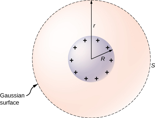
To investigate this, consider the isolated conducting sphere of Figure \(\PageIndex{9}\) that has a radius R and an excess charge q. To find the electric field both inside and outside the sphere, note that the sphere is isolated, so its surface change distribution and the electric field of that distribution are spherically symmetric. We can therefore represent the field as \(\vec{E} = E(r)\hat{r}\). To calculate \(E(r)\), we apply Gauss’s law over a closed spherical surface S of radius r that is concentric with the conducting sphere. Since \(r\) is constant and \(\hat{n} = \hat{r}\) on the sphere,
\[\begin{align} \oint \vec{E} \cdot \hat{n} \, da &= E(r) \oint da \\[4pt] &=E(r) 4\pi r^2. \end{align}\]
For \(r < R\), \(S\) is within the conductor, so recall from our previous study of Gauss’s law that \(q_{enc} = 0\) and Gauss’s law gives \(E(r) = 0\), as expected inside a conductor at equilibrium. If \(r > R\), S encloses the conductor so \(q_{enc} = q\). From Gauss’s law,
\[E(r) 4\pi r^2 = \dfrac{q}{\epsilon_0}.\]
The electric field of the sphere may therefore be written as
\[E = 0 \, (r < R),\]
and
\[E = \dfrac{1}{4 \pi \epsilon_0} \dfrac{q}{r^2} \hat{r} \, (r \geq R).\]
As expected, in the region \(r \geq R\), the electric field due to a charge q placed on an isolated conducting sphere of radius R is identical to the electric field of a point charge q located at the center of the sphere.
To find the electric potential inside and outside the sphere, note that for \(r \geq R\), the potential must be the same as that of an isolated point charge q located at \(r = 0\),
\[V(r) = \dfrac{1}{4\pi \epsilon_0} \dfrac{q}{r} (r \geq R)\]
simply due to the similarity of the electric field.
For \(r < R, \, E = 0\), so V(r) is constant in this region. Since \(V(R) = q/4\pi \epsilon_0 R\),
\[V(r) = \dfrac{1}{4 \pi \epsilon_0} \dfrac{q}{R} (r < R).\]
We will use this result to show that
\[\sigma_1 R_1 = \sigma_2 R_2,\]
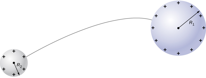
for two conducting spheres of radii \(R_1\) and \(R_2\), with surface charge densities \(\sigma_1\) and \(\sigma_2\) respectively, that are connected by a thin wire, as shown in Figure \(\PageIndex{10}\). The spheres are sufficiently separated so that each can be treated as if it were isolated (aside from the wire). Note that the connection by the wire means that this entire system must be an equipotential.
We have just seen that the electrical potential at the surface of an isolated, charged conducting sphere of radius R is
\[V = \dfrac{1}{4\pi \epsilon_0} \dfrac{q}{R}.\]
Now, the spheres are connected by a conductor and are therefore at the same potential; hence
\[\dfrac{1}{4\pi \epsilon_0} \dfrac{q_1}{R_1} = \dfrac{1}{4\pi r\epsilon_0} \dfrac{q_2}{R_2},\] and
\[\dfrac{q_1}{R_1} = \dfrac{q_2}{R_2}.\]
The net charge on a conducting sphere and its surface charge density are related by \(q = \sigma (4\pi R^2)\). Substituting this equation into the previous one, we find
\[\sigma_1 R_1 = \sigma_2 R_2.\]
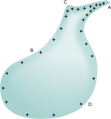
Obviously, two spheres connected by a thin wire do not constitute a typical conductor with a variable radius of curvature. Nevertheless, this result does at least provide a qualitative idea of how charge density varies over the surface of a conductor. The equation indicates that where the radius of curvature is large (points B and D in \(\PageIndex{11}\)), \(\sigma\) and E are small.
Similarly, the charges tend to be denser where the curvature of the surface is greater, as demonstrated by the charge distribution on oddly shaped metal (Figure \(\PageIndex{11}\)). The surface charge density is higher at locations with a small radius of curvature than at locations with a large radius of curvature.
A practical application of this phenomenon is the lightning rod, which is simply a grounded metal rod with a sharp end pointing upward. As positive charge accumulates in the ground due to a negatively charged cloud overhead, the electric field around the sharp point gets very large. When the field reaches a value of approximately \(3.0 \times 10^6 N/C\) (the dielectric strength of the air), the free ions in the air are accelerated to such high energies that their collisions with air molecules actually ionize the molecules. The resulting free electrons in the air then flow through the rod to Earth, thereby neutralizing some of the positive charge. This keeps the electric field between the cloud and the ground from getting large enough to produce a lightning bolt in the region around the rod.
An important application of electric fields and equipotential lines involves the heart. The heart relies on electrical signals to maintain its rhythm. The movement of electrical signals causes the chambers of the heart to contract and relax. When a person has a heart attack, the movement of these electrical signals may be disturbed. An artificial pacemaker and a defibrillator can be used to initiate the rhythm of electrical signals. The equipotential lines around the heart, the thoracic region, and the axis of the heart are useful ways of monitoring the structure and functions of the heart. An electrocardiogram (ECG) measures the small electric signals being generated during the activity of the heart.
Play around with this simulation to move point charges around on the playing field and then view the electric field, voltages, equipotential lines, and more.