5.1: Magnetic Induction

Motional EMF

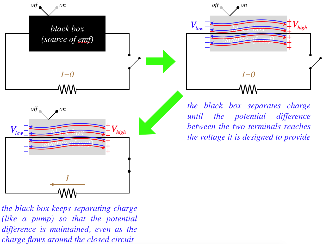
So far, our only encounter with emf has been through batteries, which separate positive and negative charge through a chemical reaction. We return now to a more general discussion of emf, so that we can apply it to what follows. To this end, let's consider an emf source that we'll describe as a black box.

Figure 5.1.1 – How Every Source of EMF Behaves

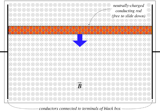
Given what we now know about magnetism, we can construct an emf source that doesn't depend upon the chemical reactions found in batteries. Suppose we replace the black box above with a pair of metal plates (across which the potential will be held at a fixed difference), with a conducting bar in contact with both that is free to slide. The other ingredient for this emf black box is a uniform magnetic field (say from a nearby bar magnet) in the region between the plates where the bar slides.

Figure 5.1.2 – New EMF Black Box

Now let's consider what happens as the bar slides down. The positive and negative charges in the bar are now moving through the magnetic field, and therefore experience magnetic forces in opposite directions. According to the right-hand-rule, positive charges will be pulled to the right, and negative charges to the left. They are confined to the conducting bar, so they cannot travel in circles – as free charges would – and end up collecting on the metal plates. They will continue to do so until the electric field of the separated charges is strong enough to oppose the magnetic forces on the charges.

Figure 5.1.3 – Motional EMF

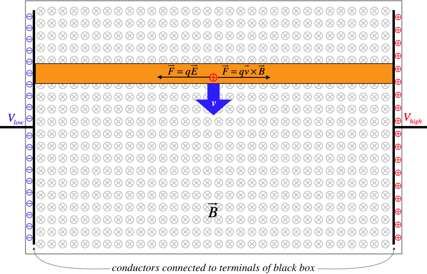
The separated charge corresponds to a potential difference between the two plates. If the terminals of this black box are used to drive a current in a circuit, the magnetic force will continue to replace the charge as long as the bar continues moving. The amount of emf produced by this device (called motional emf) can be found by computing the potential difference from the electric field that balances the force on the charges by the magnetic field:

\[\mathcal E_{motional} = EL = vBL\;,\]

where \(L\) is the length of the conducting bar.

Clearly this stores energy in the black box, but where does this energy come from? When the charges start moving along the bar, they acquire a component of motion in the horizontal direction as well as the vertical component that has been forced upon them with the motion of the bar. The positive charge moving to the right feels a force upward by the magnetic field, but it can’t leave the bar, so it pulls the bar upward (the negative charges moving in the opposite direction also pull the bar upward). This means that to keep the bar moving downward at a constant speed, a force needs to be applied from outside. This force does work on the bar (which doesn’t gain kinetic energy, since it maintains a constant speed), and this work is what adds energy to the system.

Example \(\PageIndex{1}\)

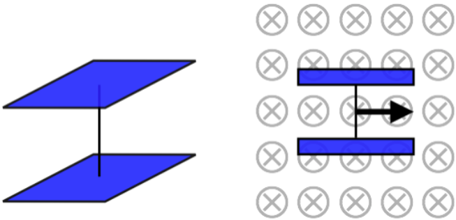
Two identical square conducting plates are oriented parallel to each other and are connected by a conducting wire as shown in the left diagram. This apparatus is then moved through a uniform magnetic field as shown in the right diagram (the thickness of the plates is negligible). The strength of the magnetic field is \(1.5T\). The apparatus is moving at a speed of \(8.0\frac{m}{s}\). Find the uniform charge density (including its sign) induced on the top plate.

Solution

Motional emf will create a potential difference between the two ends of the wire, which means there will be a potential difference between the two conducting plates. Once the steady potential difference is established, this essentially becomes a charged parallel-plate capacitor. Setting the motional emf equal to the potential difference between capacitor plates, gives:

\[\left. \begin{array}{l}\mathcal E_{motional} = Bvd \\ V_{capacitor} = \dfrac{Q}{C} \\ C_{parallel-plate} \end{array} \right\} \;\;\; Bvd = \dfrac{Q}{C}=\dfrac{Qd}{A\epsilon_o} \nonumber\]

The ratio \(\frac{Q}{A}\) is the charge density, so we can immediately compute its magnitude:

\[\sigma = \dfrac{Q}{A} = \epsilon_oBv = \left(8.85\times 10^{-12}\frac{C^2}{N\cdot m^2}\right)\left(1.5T\right)\left(8.0\frac{m}{s}\right) = 1.1\times 10^{-10}\frac{C}{m^2}\nonumber\]

With the plates moving to the right and the magnetic field into the page, the RHR shows that positive charges in the wire will feel a force upward, which means the top plate will be positively charged.

[It should be noted that one does not need to treat this as a parallel plate capacitor to achieve this answer. The charges stop flowing when the magnetic force balances the electric field force created by the separated charges. This electric field is, to a good approximation (the same one we make for parallel-plate capacitors), uniform between the plates, and at each plate the magnitude is \(\frac{\sigma}{\epsilon_o}\). This achieves the same answer.]

Faraday's Law

Now that we know we can generate emf in conductors using magnetic fields, we will explore this phenomenon further. We’ll start by looking at an alternate way of describing the phenomenon of motional emf that comes courtesy of a fellow named Michael Faraday, who did his work in this area in the middle of the 19th century.

Instead of stopping the analysis of the moving bar at the boundaries of the black box, let's include the entire circuit. When we do this, the magnetic field passes through a closed loop defined by the circuit, and we can write the magnetically-induced emf in terms of the magnetic flux \(\Phi_B\) through that closed loop.

Figure 5.1.4 – Faraday's Model for Magnetically-Induced EMF

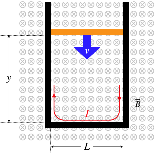
The emf induced in this physical system needs to be the same as it was above, and Faraday noted that the magnitude of the emf can be computed in terms of the time rate of change of the magnetic flux through the closed loop:

\[\Phi_B = \int \overrightarrow B\cdot d\overrightarrow A = BLy \;\;\;\Rightarrow\;\;\; \left|\mathcal E\right| = \left|vBL\right|=\left|-\dfrac{dy}{dt}BL\right|=\left|\dfrac{d}{dt}\left(BLy\right)\right|=\left|\dfrac{d\Phi_B}{dt}\right|\]

This may seem like a pointless rewriting of the motional emf result we got above, but in fact this turns out to be the more general rule for magnetically-induced emf. That is, there are more ways than just moving one of the sides of a rectangle to change the flux through a loop. Before we go into details of some of these variants, we need to take a moment to clarify what is meant by an emf being induced in a closed loop.

For the example given above, the potential difference created is obvious – the right side of the sliding bar is at a higher potential than the left side.

Figure 5.1.5 – Kirchhoff Loop Rule Applied to Sliding Bar Case

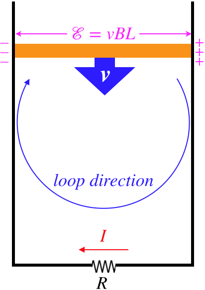
This means that if we employ Kirchhoff's loop rule to this circuit, we get:

\[+\mathcal E-IR=0\]

But Faraday's formulation of induced emf does not require a moving bar. For example, if the dimensions of the circuit don't change at all, the magnetic flux can still be changed by altering the magnetic field. If we try to do the same thing as above with Kirchhoff's loop rule, we don't have a specific segment of the loop where the potential jumps, so how do we account for the induced emf? Faraday's answer is that we simply modify Kirchhoff's loop rule – instead of having the sum of the voltage drops around the loop adding up to zero, they add up to the contribution of the changing magnetic flux:

\[sum\;of\;voltage\;drops\;around\;closed\;loop = \dfrac{d\Phi_B}{dt} = \dfrac{d}{dt}\int\limits_{\;\;\;area\\defined\;by \\closed\;loop}\overrightarrow B \cdot d\overrightarrow A\]

There is only one tricky detail left to clarify here – the sign convention. The area vector for the flux calculation is defined by the closed loop, but this vector needs a direction, and there are two possible directions to choose from. This direction is defined by our chosen loop direction and (what else?) the right-hand rule, in the same way that we defined the direction of the area vector for the magnetic moment; curl the fingers to trace the loop direction, and thumb points the direction of the area vector.

Let's try this for the case given above. The loop direction is clockwise, giving an area vector into the page. The magnetic field is also into the page, so the flux is a positive value. This flux is decreasing with time, which means that the time derivative of the flux is negative, giving for our modified Kirchhoff loop rule:

\[-IR = \dfrac{d}{dt}\int\overrightarrow B \cdot d\overrightarrow A = \dfrac{d}{dt}\left(+BLy\right) = Bx\dfrac{dy}{dt} = BL\left(-v\right)\]

If we had chosen the loop direction to be counterclockwise, then the voltage change across the resistor would be positive (because the labeled direction of the current is opposite to the loop direction), and the flux would be negative, giving the same final result. Typically this is expressed in terms of the emf that needs to be added into the Kirchhoff loop to again give a zero loop sum. That is:

\[sum\;of\;voltage\;drops\;around\;closed\;loop + \mathcal E_{induced}= 0 \;\;\;\Rightarrow\;\;\; \mathcal E_{induced} =-\dfrac{d\Phi_B}{dt} \]

There is one more detail that needs to be added here. If the circuit consists of a coil of wire with many (\(N\)) turns in it, then the flux through every turn contributes to the induced emf, giving the final form of what is known as Faraday's law:

\[\mathcal E_{induced} =-N\dfrac{d\Phi_B}{dt} \]

Lenz's Law

Keeping track of the sign convention in Ampére's law can be an odious task, but it turns out there is an easier way to determine the direction that the induced emf would seek to drive a current. Not only is it easier, but it provides some useful physical insight into why the minus sign appears in Faraday's law.

Suppose we have a closed loop of conducting wire in the plane of this page, through which we suddenly introduce a magnetic field into the page. This change in magnetic flux will induce an emf in the loop, which will in turn result in a current flowing through the loop. Which way will this current flow? A Russian physicist named Emil Lenz argued that the current would have to be induced counterclockwise, for the following reason: The induced current will contribute to the total magnetic field passing through the loop (magnetic dipoles also have fields!), and if the induced current was clockwise, then the additional field from the current in the wire would increase the flux that has already been increased. This would induce more current in the same direction, which would induce more current, and so on. Obviously the energy in the circuit would then grow without bound, which isn't possible. He therefore landed upon what is now known as Lenz's Law:

The emf induced in a circuit will be such that a current resulting from it will produce a secondary magnetic flux that seeks to undo the change in flux that induced the emf in the first place.

It should be noted that induced emf's don't always drive a current (e.g. there may be a battery present, and the induced emf may only slow the current), but it is not the resulting current that matters – the induced emf will "try" to induce a current in a direction that counters the change in flux. Also, the amount of current induced generally will not entirely undo the change in flux – this law only provides the direction of the induced emf.

An Illustrative Example

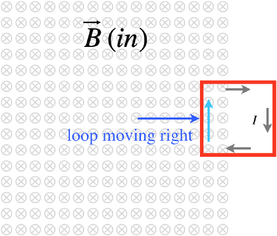
It is useful to look at a few concrete examples of magnetic induction. The first involves a closed conducting loop moving through a region of uniform magnetic field. In this case, we can view it either in terms of Faraday's law, or in terms of motional emf.

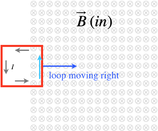
Figure 5.1.6 – Conducting Loop Enters Uniform Magnetic Field

Motional EMF Explanation

When the loop first enters the field, only the right side of the loop is moving through the field, so the motional emf creates a higher potential at the top of this side than at the bottom. The imbalance drives a current counterclockwise.

Faraday/Lenz Explanation

As the loop enters the field, the magnetic flux through it increases into the page. This induces an emf that seeks to drive a current whose magnetic field will oppose this change. To reduce the flux inward, a field needs to be created that points out of the page inside the loop. From the right-hand-rule, this requires a counterclockwise current.

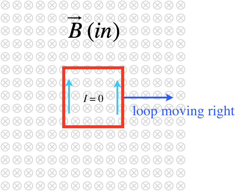
Figure 5.1.7 – Conducting Loop Stays Within the Uniform Magnetic Field

Motional EMF Explanation

With the loop entirely within the field, both the left and right sides of the loop exhibit motional emf, holding the top segment of the loop at a higher potential than the bottom segment. But just as if two identical batteries were placed in both sides of the circuit with their positive terminals facing up, this does not result in any current around the loop.

Faraday/Lenz Explanation

As the loop remains within the uniform field, the flux through the loop doesn't change, because none of the factors that goes into the calculation of the flux changes. With an unchanging flux, there is no induced emf in the loop, and no current as a result.

Figure 5.1.8 – Conducting Loop Exits the Uniform Magnetic Field

Motional EMF Explanation

Once again the loop has one of its sides outside the field, so only one side exhibits motional emf. This again results in an imbalance that drives a current. In this case, the current is in the opposite direction as when the loop entered the field.

Faraday/Lenz Explanation

The loop is losing inward flux with time as it leaves the field, so the emf induced will act to create a current that opposes this loss of flux. The direction of the current that will bolster the field inside the loop into the page is clockwise.

Not withstanding this enlightening example, we can't handle every case by resorting to a motional emf argument. For emf to be induced, we only need that the flux through a closed loop changes. Given the definition of the flux, there are many ways for this to happen:

\[\Phi_B=\int\overrightarrow B \cdot d\overrightarrow A = \int BdA\cos\theta\]

• area changing with time (e.g. sliding bar example earlier)
• magnetic field changing with time (e.g. move a magnet farther or closer to change the field strength)
• change the angle \(\theta\) between the field and the area (e.g. a rotating loop in a uniform field)
• change the the integral (e.g. move the loop between regions where the magnetic field is different).
• any combination of the above

When we calculate the flux, we need to add up the small flux increments over the whole surface… But what surface? While we tend to think of the surface as being the flat area defined by the loop, there are actually infinitely-many surfaces defined by the loop as a border. Well, it turns out that all of the surfaces result in the same flux, for the following reason: Consider two different surfaces at once: The flux that goes through one, must go out of the other one (since they are bordered by the same closed loop), because as we know from Gauss’s Law for magnetism, the magnetic flux for any closed surface is zero (no magnetic monopoles). Therefore the flux through every surface defined by the boundary is the same.

Example \(\PageIndex{2}\)

A square loop of wire with a total resistance \(R\) has a side-length of \(L\). It resides near a long, straight wire such that the long wire is in the same plane as the loop, with one of its sides parallel to the wire a distance d from it, as shown in the diagram.

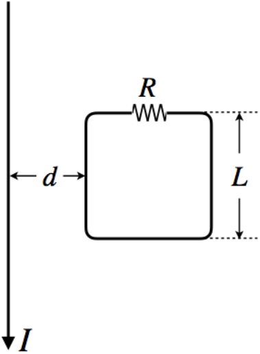
1. Compute the magnetic flux through the loop due to a current \(I\) flowing in the direction shown in the diagram.
2. If the current in the long wire is changing, then the magnetic field flux through the loop will also be changing. Suppose that the current in the long wire is increasing at a constant rate of \(\frac{dI}{dt}=\alpha\). Find the current induced in the loop, including its direction.

Solution

a. We know the magnetic field for a long-straight wire gets weaker at greater distances, which means we have to perform the flux integral. The diagram below shows the magnetic field and introduces some axes for performing the math required.

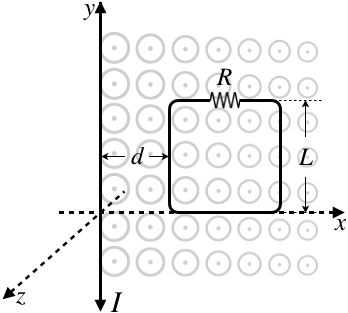
The magnetic field strength in the \(x\)-\(y\) plane in terms of the distance \(x\) from the long wire is given by:

\[B = \dfrac{\mu_oI}{2\pi x} \nonumber\]

We take as a differential area element a thin vertical slice down the length of the circuit. This slice has an area of \(dA = Ldx\), and the field is constant throughout the slice. Also, the area vector is parallel to the magnetic field, so choosing the loop direction as counterclockwise, the angle between the field and the area vector is \(0^o\). The flux integral is therefore:

\[\Phi_B = \int \overrightarrow B \cdot d\overrightarrow A = \int BdA\cos\theta = \int\limits_{x=d}^{x=d+L}\left(\dfrac{\mu_oI}{2\pi x}\right)Ldx\cos0^o = \dfrac{\mu_oIL}{2\pi}\ln\left[\dfrac{d+L}{d}\right]\nonumber\]

b. The emf induced in the loop (which has only one turn in it) is found using Faraday's law:

\[\mathcal E_{induced} = -\dfrac{d\Phi_B}{dt} = -\dfrac{\mu_oL}{2\pi}\ln\left[\dfrac{d+L}{d}\right]\dfrac{dI}{dt} = -\dfrac{\mu_oL\alpha}{2\pi}\ln\left[\dfrac{d+L}{d}\right] \nonumber\]

The magnitude of the current is this emf divided by the resistance:

\[\dfrac{\mu_oL\alpha}{2\pi R}\ln\left[\dfrac{d+L}{d}\right]\nonumber\]

The direction of the current will be such that it provides a field that will seek to counter the change. The current that is causing the field is increasing, so the flux out of the page in increasing. The induced current will therefore produce a magnetic field inside the loop that points into the page, which means it must flow clockwise.