5.3: Inductance

Mutual Inductance

In keeping with our tradition of following the lead from electricity when discussing magnetism (Coulomb vs. Biot-Savart, dipole math, Gauss vs. Ampére, etc.), it’s time we tackled magnetism’s version of capacitance. Just to review, capacitance was purely a static charge notion – a way of storing energy on two conductors that hold opposite charges. Magnetism is anything but a static charge phenomenon, so its version of capacitance will have to be quite different. It is different, but there are many parallels as well.

If we place two circuits near each other and change the current flowing through one of them, then the magnetic field for that changing current will also change. If this magnetic field results in a flux through the second circuit, then its change can induce a current in the second circuit. So somehow we can transfer energy from one circuit to another without the circuits even being connected to each other. One way to explain this is to assume that there is energy present in the magnetic field itself. We already know that energy is contained in an electric field, so this is not a surprising revelation. Here's a diagram of this physical situation:

Figure 5.3.1 – Mutual Inductance

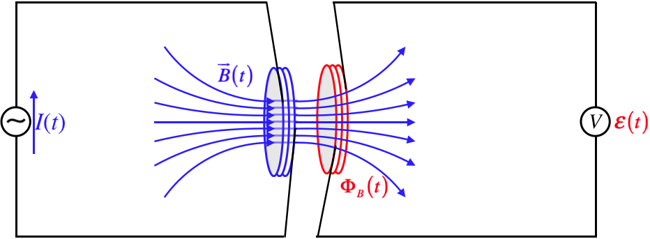
We have introduced a new symbol here. The circle with the wavy line indicates a variable current source (this explains why there is the time-dependent current variable right next to it). This variable current \(I\left(t\right)\) passes through the left coil, resulting in a time-dependent magnetic field \(\overrightarrow B\left(t\right)\). This field passes through the right coil, resulting in a time-varying flux \(\Phi_B\left(t\right)\). Faraday's law says that this variable flux results in an induced emf \(\mathcal E \left(t\right)\) registered in the voltmeter.

Our goal here is to mathematically relate the emf developed in the secondary coil to the variable current sent through the primary coil. We start by noting that the magnetic field strength is directly proportional to the current through the primary coil (the one on the left in the figure above), and the magnetic flux through the secondary coil is proportional to the magnetic field strength. Both of these facts are based on the idea that the field and its relation to the area through which it passes has the same shape, given that the geometry of the construction of this device remains unchanged. This should sound very familiar. Putting these proportionalities together, we get that the flux through the secondary coil (which we'll say has \(N\) turns) is proportional to the current through the primary coil, and we can define a proportionality constant \(M\), called the mutual inductance of the construction:

\[N\Phi_B\left(t\right) =M I\left(t\right)\]

This gives us the relationship between the input current and the resulting emf that we were looking for, from Faraday's law:

\[\mathcal E\left(t\right) = -M\dfrac{d}{dt}I\left(t\right)\]

This is the magnetic analog to the electrostatic \(Q=CV\). Like the case of capacitance, the mutual inductance is only a function of how the device is constructed – it doesn't change when the current through it is changed, just as capacitance is not changed by altering the amount of charge on the plates. The units for inductance are:

\(\left[M\right] = \left[\dfrac{B\cdot A}{I}\right] = \dfrac{T\cdot m^2}{A} \equiv H\;\;\; \text{("henry")}\)

One thing that seems to distinguish mutual inductance from capacitance is the apparent one-way nature of it – there are distinct primary and secondary coils, while a capacitor just has two conductors, either of which can take the positive charge. Well, it turns out that mutual inductance is equally reversible! The reason is that the number of turns in the primary coil is proportional to the magnetic field strength in the same way that the number of turns in the secondary coil is proportional to the total flux. That is, if we swap the current source and the voltmeter in the figure above, we get the same result. We can express this mathematically by labelling everything (number of turns, flux, and current) for each coil differently:

\[M=\dfrac{N_2\Phi_2}{I_1} = \dfrac{N_1\Phi_1}{I_2}\]

Let's see that this is true (as well as explore some nuances of the physics) by looking at an example. The physical setup consists of two coaxial solenoids of equal lengths, but their own cross-sectional areas and number of turns.

Figure 5.3.2 – Mutual Inductance of Coaxial Solenoids – Outer Cylinder Carries Current

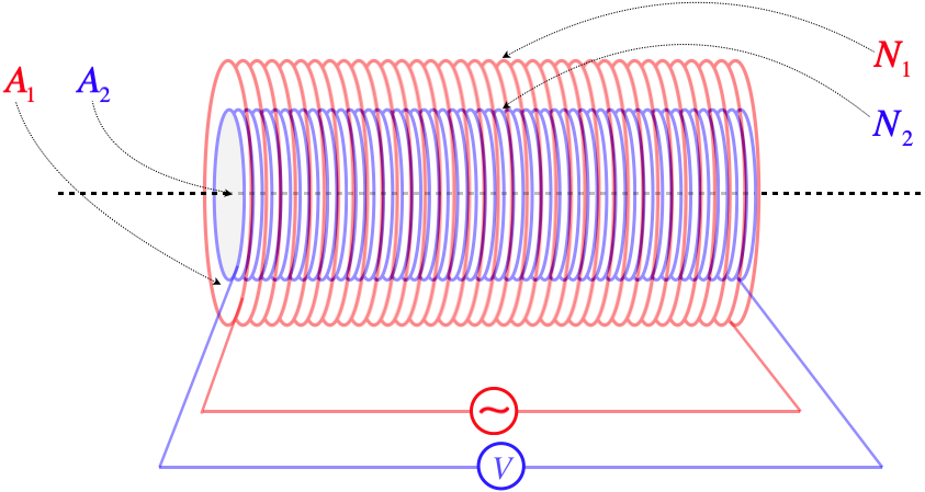
In this setup, we have the applied varying current going through the outside solenoid, and the changing flux within the inside solenoid. The outer solenoid's field is uniform throughout its interior, and only the portion within the region of the inner solenoid contributes to the flux.

Figure 5.3.3 – Flux Through Inner Solenoid of Field from Outer Solenoid

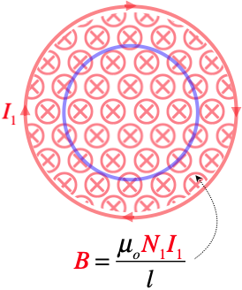
The field produced by the outer solenoid is easily calculable from the current, the number of turns, and the length, and the flux is easy to calculate from there:

\[\Phi_2 = BA_2 = \left(\dfrac{\mu_oN_1I_1}{l}\right)A_2\;\;\;\Rightarrow\;\;\; M=\dfrac{N_2\Phi_2}{I_1} = \dfrac{\mu_oN_1N_2A_2}{l}\]

We can see that this result depends only upon the structure of the two solenoids. Okay, so let's check to see if the reversibility property holds. We now put the varying current through the inner solenoid.

Figure 5.3.4 – Mutual Inductance of Coaxial Solenoids – Inner Cylinder Carries Current

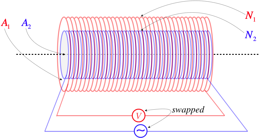
As before, we need to determine the flux through the secondary coil due to the current in the primary, but this time the picture is slightly different.

Figure 5.3.5 – Flux Through Outer Solenoid of Field from Inner Solenoid

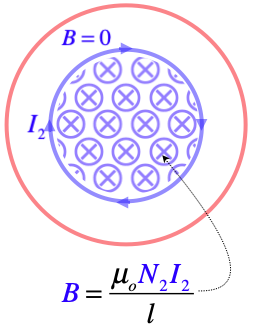
The flux through the outer solenoid comes in two parts: The flux through the central region due to the field inside the inner solenoid, and zero flux through the outer region:

\[\Phi_1=B_{inner}A_2 + B_{outer}\left(A_1-A_2\right) = \left(\dfrac{\mu_oN_2I_2}{l}\right)A_2+0 = \dfrac{\mu_oN_2I_2A_2}{l}\]

Now plug this into the definition of mutual inductance and find that it is the same as when the roles of the solenoids were reversed:

\[M=\dfrac{N_1\Phi_1}{I_2} = \dfrac{\mu_oN_1N_2A_2}{l}\]

Self-Inductance

We can now see how one circuit can affect another without being in physical contact, but in fact there really doesn’t need to be two coils in order to witness an effect of magnetic induction. Suppose we have a varying current in a circuit containing a single solenoid. As the current in the solenoid varies, the magnetic field inside the solenoid changes, which in turn changes the magnetic flux through that same solenoid. That induces an emf across the solenoid, which will in turn have an effect on the current through it! This process is known as self-inductance.
We actually define self-inductance in the same way that we defined mutual inductance – the ratio of the total flux through the \(N\) coils to the current that supplies the magnetic field. Naturally the units are therefore the same as mutual inductance.

\[L\equiv\dfrac{N\Phi}{I}\]

In practical terms, the only reasonable device for which we can compute the self-inductance is a solenoid, as its uniform magnetic field makes the flux easy to compute:

\[L_{solenoid}=\dfrac{N\Phi}{I} = \dfrac{N\left(BA\right)}{I} = \dfrac{N\left(\dfrac{\mu_oNI}{l}\right)A}{I} = \dfrac{\mu_oN^2A}{l}\]

As with mutual inductance, this value \(L\) is a constant that depends only upon the structure of the solenoid (hereafter referred to as an inductor). The difference here of course is that the emf induced by the current/field/flux change acts to affect the same current that causes the flux change to begin with. In particular:

\[N\Phi = LI \;\;\;\Rightarrow\;\;\; N\dfrac{d}{dt}\Phi = \dfrac{d}{dt}\left(LI\right) \;\;\;\Rightarrow\;\;\; \mathcal E = -N\dfrac{d}{dt}\Phi=-L\dfrac{d}{dt}I\]

How do we interpret this? Think back to what is happening here – Faraday’s law is in play, and this means that an emf is induced (like a battery, but without the chemical reaction). So we can think of this as a “smart battery” that adjusts its emf (magnitude and direction) according to what is happening to the current. The minus sign indicates that this smart battery adjusts itself to oppose changes. If the current is dying down, the inductor comes to the rescue and provides an emf to try to help maintain the current, and if the current is growing, then the inductor provides an emf to try to slow the increase.

Figure 5.3.6 – Inductor Behaves Like a "Smart Battery"

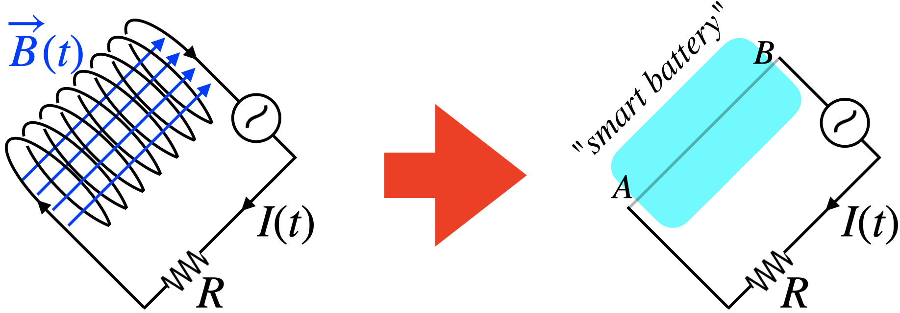
In the figure above, if the current is dying-down, the magnitude of the magnetic field diminishes, reducing the flux through the inductor. The induced emf across the inductor will be such that it will seek to bolster the current through itself (which also goes through the resistor). This requires that the potential at terminal \(B\) of the smart battery be greater than the potential at terminal \(A\). If the current is increasing, then to fight this change, the potential of terminal \(A\) of the smart battery must be greater than the potential at terminal \(B\).

Let's use Kirchhoff's loop rule on this circuit. Choosing a loop direction of clockwise, we have:

\[V_B-V_A -IR = 0\]

If the current is decreasing, then its derivative is negative. In this case, the inductor acts like a smart battery with its positive terminal at position \(B\), so the voltage drop across the inductor for our clockwise loop needs to be positive. If the current is instead increasing, then the derivative of the current is positive, and the smart battery reverses direction, making the voltage drop across the inductor for the clockwise loop negative. Both of these scenarios are in agreement with the conclusion above that the potential drop across an inductor satisfies \(\mathcal E = -L\frac{dI}{dt}\).