
5.4: Inductors in Circuits
- Page ID
- 21537

\( \newcommand{\vecs}[1]{\overset { \scriptstyle \rightharpoonup} {\mathbf{#1}} } \)
\( \newcommand{\vecd}[1]{\overset{-\!-\!\rightharpoonup}{\vphantom{a}\smash {#1}}} \)
\( \newcommand{\dsum}{\displaystyle\sum\limits} \)
\( \newcommand{\dint}{\displaystyle\int\limits} \)
\( \newcommand{\dlim}{\displaystyle\lim\limits} \)
\( \newcommand{\id}{\mathrm{id}}\) \( \newcommand{\Span}{\mathrm{span}}\)
( \newcommand{\kernel}{\mathrm{null}\,}\) \( \newcommand{\range}{\mathrm{range}\,}\)
\( \newcommand{\RealPart}{\mathrm{Re}}\) \( \newcommand{\ImaginaryPart}{\mathrm{Im}}\)
\( \newcommand{\Argument}{\mathrm{Arg}}\) \( \newcommand{\norm}[1]{\| #1 \|}\)
\( \newcommand{\inner}[2]{\langle #1, #2 \rangle}\)
\( \newcommand{\Span}{\mathrm{span}}\)
\( \newcommand{\id}{\mathrm{id}}\)
\( \newcommand{\Span}{\mathrm{span}}\)
\( \newcommand{\kernel}{\mathrm{null}\,}\)
\( \newcommand{\range}{\mathrm{range}\,}\)
\( \newcommand{\RealPart}{\mathrm{Re}}\)
\( \newcommand{\ImaginaryPart}{\mathrm{Im}}\)
\( \newcommand{\Argument}{\mathrm{Arg}}\)
\( \newcommand{\norm}[1]{\| #1 \|}\)
\( \newcommand{\inner}[2]{\langle #1, #2 \rangle}\)
\( \newcommand{\Span}{\mathrm{span}}\) \( \newcommand{\AA}{\unicode[.8,0]{x212B}}\)
\( \newcommand{\vectorA}[1]{\vec{#1}} % arrow\)
\( \newcommand{\vectorAt}[1]{\vec{\text{#1}}} % arrow\)
\( \newcommand{\vectorB}[1]{\overset { \scriptstyle \rightharpoonup} {\mathbf{#1}} } \)
\( \newcommand{\vectorC}[1]{\textbf{#1}} \)
\( \newcommand{\vectorD}[1]{\overrightarrow{#1}} \)
\( \newcommand{\vectorDt}[1]{\overrightarrow{\text{#1}}} \)
\( \newcommand{\vectE}[1]{\overset{-\!-\!\rightharpoonup}{\vphantom{a}\smash{\mathbf {#1}}}} \)
\( \newcommand{\vecs}[1]{\overset { \scriptstyle \rightharpoonup} {\mathbf{#1}} } \)
\(\newcommand{\longvect}{\overrightarrow}\)
\( \newcommand{\vecd}[1]{\overset{-\!-\!\rightharpoonup}{\vphantom{a}\smash {#1}}} \)
\(\newcommand{\avec}{\mathbf a}\) \(\newcommand{\bvec}{\mathbf b}\) \(\newcommand{\cvec}{\mathbf c}\) \(\newcommand{\dvec}{\mathbf d}\) \(\newcommand{\dtil}{\widetilde{\mathbf d}}\) \(\newcommand{\evec}{\mathbf e}\) \(\newcommand{\fvec}{\mathbf f}\) \(\newcommand{\nvec}{\mathbf n}\) \(\newcommand{\pvec}{\mathbf p}\) \(\newcommand{\qvec}{\mathbf q}\) \(\newcommand{\svec}{\mathbf s}\) \(\newcommand{\tvec}{\mathbf t}\) \(\newcommand{\uvec}{\mathbf u}\) \(\newcommand{\vvec}{\mathbf v}\) \(\newcommand{\wvec}{\mathbf w}\) \(\newcommand{\xvec}{\mathbf x}\) \(\newcommand{\yvec}{\mathbf y}\) \(\newcommand{\zvec}{\mathbf z}\) \(\newcommand{\rvec}{\mathbf r}\) \(\newcommand{\mvec}{\mathbf m}\) \(\newcommand{\zerovec}{\mathbf 0}\) \(\newcommand{\onevec}{\mathbf 1}\) \(\newcommand{\real}{\mathbb R}\) \(\newcommand{\twovec}[2]{\left[\begin{array}{r}#1 \\ #2 \end{array}\right]}\) \(\newcommand{\ctwovec}[2]{\left[\begin{array}{c}#1 \\ #2 \end{array}\right]}\) \(\newcommand{\threevec}[3]{\left[\begin{array}{r}#1 \\ #2 \\ #3 \end{array}\right]}\) \(\newcommand{\cthreevec}[3]{\left[\begin{array}{c}#1 \\ #2 \\ #3 \end{array}\right]}\) \(\newcommand{\fourvec}[4]{\left[\begin{array}{r}#1 \\ #2 \\ #3 \\ #4 \end{array}\right]}\) \(\newcommand{\cfourvec}[4]{\left[\begin{array}{c}#1 \\ #2 \\ #3 \\ #4 \end{array}\right]}\) \(\newcommand{\fivevec}[5]{\left[\begin{array}{r}#1 \\ #2 \\ #3 \\ #4 \\ #5 \\ \end{array}\right]}\) \(\newcommand{\cfivevec}[5]{\left[\begin{array}{c}#1 \\ #2 \\ #3 \\ #4 \\ #5 \\ \end{array}\right]}\) \(\newcommand{\mattwo}[4]{\left[\begin{array}{rr}#1 \amp #2 \\ #3 \amp #4 \\ \end{array}\right]}\) \(\newcommand{\laspan}[1]{\text{Span}\{#1\}}\) \(\newcommand{\bcal}{\cal B}\) \(\newcommand{\ccal}{\cal C}\) \(\newcommand{\scal}{\cal S}\) \(\newcommand{\wcal}{\cal W}\) \(\newcommand{\ecal}{\cal E}\) \(\newcommand{\coords}[2]{\left\{#1\right\}_{#2}}\) \(\newcommand{\gray}[1]{\color{gray}{#1}}\) \(\newcommand{\lgray}[1]{\color{lightgray}{#1}}\) \(\newcommand{\rank}{\operatorname{rank}}\) \(\newcommand{\row}{\text{Row}}\) \(\newcommand{\col}{\text{Col}}\) \(\renewcommand{\row}{\text{Row}}\) \(\newcommand{\nul}{\text{Nul}}\) \(\newcommand{\var}{\text{Var}}\) \(\newcommand{\corr}{\text{corr}}\) \(\newcommand{\len}[1]{\left|#1\right|}\) \(\newcommand{\bbar}{\overline{\bvec}}\) \(\newcommand{\bhat}{\widehat{\bvec}}\) \(\newcommand{\bperp}{\bvec^\perp}\) \(\newcommand{\xhat}{\widehat{\xvec}}\) \(\newcommand{\vhat}{\widehat{\vvec}}\) \(\newcommand{\uhat}{\widehat{\uvec}}\) \(\newcommand{\what}{\widehat{\wvec}}\) \(\newcommand{\Sighat}{\widehat{\Sigma}}\) \(\newcommand{\lt}{<}\) \(\newcommand{\gt}{>}\) \(\newcommand{\amp}{&}\) \(\definecolor{fillinmathshade}{gray}{0.9}\)Magnetic Field Energy
Inductors are what we were looking for – a device that goes into a circuit like a capacitor which involves magnetic rather than electric fields. Several chapters ago, we said that the primary purpose of a capacitor is to store energy in the electric field between the plates, so to follow our parallel course, the inductor must store energy in its magnetic field. We can calculate exactly how much is stored using tools we already have.
Suppose we start building up a current from zero into an inductor. With no current in it, there is no magnetic field and therefore zero energy, but as the current rises, the magnetic field grows, and the energy stored grows with it. We actually have a way of determining the rate at which the energy stored is growing from what we know already. There is no resistance to worry about here, so none of the energy is lost to thermal, which means that we can write the power as the product of the current and the voltage difference. As a reminder, power delivered to or by a battery is plus-or-minus the product of the current and the emf of the battery:
Figure 5.4.1 – Power Charging or Discharging a Battery
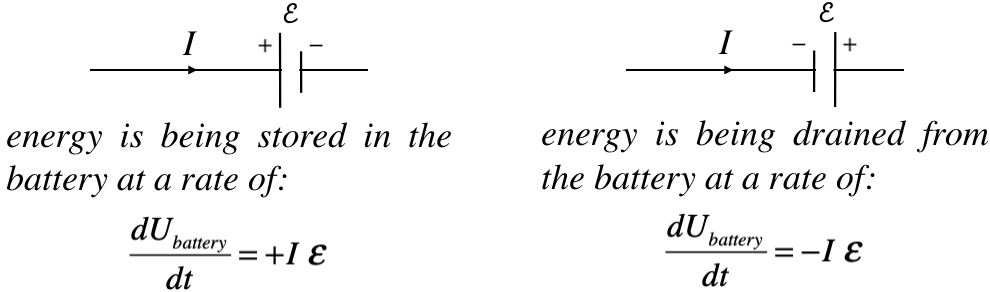
With the idea of an inductor behaving like a smart battery, we have method of determining the rate at which energy is accumulated within (or drained from) the magnetic field within the inductor. If the positive lead of our smart battery is facing the incoming current, it must be because the current is increasing. This results in an increase in the energy stored in the inductor, and sure enough, an increase in current corresponds to an increase in the magnetic field strength within the inductor. The reverse argument for an inductor where the current (and therefore field) is decreasing also fits perfectly. The math works easily by replacing the emf of the battery with that of an inductor:
\[\dfrac{dU_{inductor}}{dt} = I\left(L\dfrac{dI}{dt}\right)=LI\dfrac{dI}{dt}\]
We can now determine the energy within the inductor by integrating this power over time:
\[U_{inductor} = \int Pdt = \int \left(LI\dfrac{dI}{dt}\right)dt = L\int IdI = \frac{1}{2} LI^2\]
There is clearly a resemblance of this energy to that of a charged capacitor, though the parallels are not immediately obvious. It seems reasonable to relate the charge to the current, because in each case, these are what is accumulated within the device. This would mean that the parallel between capacitance and self-inductance is \(C\leftrightarrow L^{-1}\). This parallel only goes so far, however. For example, it doesn't work for \(Q=CV\). For energy considerations, however, it does work well, and we will see that this extends to field energy.
The potential energy stored within a solenoid (which, as we stated above, is pretty much the design of every inductor) can be written in terms of the magnetic field within. For this we need the self-inductance of a solenoid (Equation 5.3.8), and the field of a solenoid (Equation 4.4.13):
\[U_{solenoid} = \frac{1}{2}LI^2 = \frac{1}{2}\left(\dfrac{\mu_oN^2A}{l}\right)I^2 = \dfrac{1}{2\mu_o}\left(\dfrac{\mu_oNI}{l}\right)^2\left(A\cdot l\right) = \dfrac{1}{2\mu_o}B^2\left(A\cdot l\right)\]
The quantity \(A\cdot l\) is the volume of the solenoid, so dividing both sides by this gives the energy density of the magnetic field within the solenoid:
\[u_{solenoid} = \dfrac{U_{solenoid}}{volume} = \dfrac{1}{2\mu_o}B^2\]
Once again, the resemblance with the electric field version is clear, with the only difference being that the constant appears in the denominator here, while its electric counterpart appears in the numerator.
Enhancing Inductors
When we discussed capacitors, we found that we could alter their energy-storing capabilities by putting a dielectric between their plates. We have a similar option for inductors. We previously discussed the concepts related to magnetic fields in various substances, learning that substances can react in basically one of two ways: The magnetic dipoles in the substance can align with the field, or new dipoles can be induced which (according to Lenz’s law) align opposite to the field. The former we called paramagnetism (or, if the dipoles remain aligned after removing the field, ferromagnetism) and it augments the applied field. The latter we called diamagnetism, and it reduces the applied field. This contrasts with the case of electricity, where insulating materials can only react as dielectrics, and only act to reduce the field.
As in the case of electricity, we will introduce a physical constant known as the permeability, which, like the permittivity in the case of electricity, takes the place of the vacuum constant:
\[\text{electricity: } \epsilon_o \rightarrow \epsilon \;\;\;\;\;\;\;\; \text{magnetism: }\mu_o \rightarrow \mu \]
As with the case of electricity, we simply replace the vacuum permeability with the permeability of the substance to get the answers inside of matter. So Biot-Savart and Ampére’s laws are easily translated into more general forms:
\[\overrightarrow B = \dfrac{\mu}{4\pi}\int\dfrac{I\overrightarrow {dl} \times \widehat r}{r^2}\;\;\;\;\;\;\;\;\oint \overrightarrow B \cdot \overrightarrow {dl} = \mu I_{enclosed}\]
Notice from Biot-Savart's law that increasing the permeability for the same source increases the field strength (contrast this with the permittivity in the case of the Coulomb field). Therefore a permeability higher than the vacuum means the material is paramagnetic (and much higher than that is ferromagnetic). A value lower than the vacuum value corresponds to diamagnetism. Frequently materials are classified according to the percentage increase/decrease they provide to the total field compared to the vacuum case. That is:
\[\mu = \left(1+\chi_m\right)\mu_o\]
The constant \(\chi_m\) is called the magnetic susceptibility. This has a positive for substances that are paramagnetic and ferromagnetic, and a negative value for diamagnetic substances.
LR Circuits
It's time to add inductors into our circuit diagrams, so we need a new symbol:
inductor: 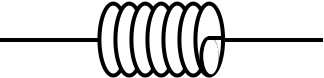
As with any other object in a circuit, there will be a specific voltage drop across the device as we invoke Kirchhoff’s loop rule. The difference with this device it that its “smart battery” property makes it somewhat trickier than the other objects to determine the sign of the voltage change.
One reason to include an inductor in a circuit is to protect the circuit from current spikes (i.e. as a surge protector). If the current changes dramatically and suddenly, then the inductor will respond by providing an emf that opposes the sudden change, reducing the amount that the current is able to change over a short period, protecting the system from potential damage. We will see some other effects that an inductor has on a circuit as well, starting with how it interacts in a circuit with a resistor.
Figure 5.4.2a – An LR Circuit with Growing Current
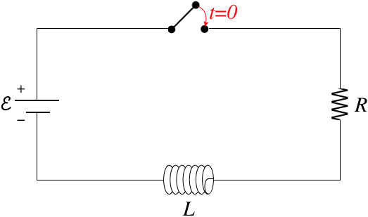
When the switch is first closed, the current "wants" to jump instantly from zero to satisfy \(\mathcal E = IR\), but the inductor doesn’t allow this, because it develops an emf to oppose sudden changes. We begin with the Kirchhoff loop rule (which provides a new challenge for us when it comes to inductors), then solve the differential equation as we did for the RC circuit previously. To use the loop rule, we need to label a current and choose a loop direction. For the case above, let's choose clockwise for both. Going around this loop, the battery provides a voltage increase of \(+\mathcal E\), and the resistor a voltage drop of \(-IR\). What about the inductor?
When the switch is closed, the current that points right-to-left for the inductor increases in the direction of the loop. As a result of Faraday's law, the inductor becomes a "smart battery" that acts to reduce the current, which means there is a voltage drop:
\[\mathcal E_{inductor} = -L\dfrac{dI}{dt}\]
With the current increasing, the derivative is positive, and since \(L\) is always positive, a voltage drop requires a minus sign. Before we put the loop equation together, let's ask how this might change if we had labeled the current differently or chosen a different loop direction. First, if we switch the direction of the current label to left-to-right, and leave the loop direction, then an increasing current will result in the left side of the "smart battery" being at higher potential, which means that in a clockwise loop, the inductor would give a potential increase, and we would have to use \(\mathcal E_{inductor} = +L\dfrac{dI}{dt}\). So it seems clear that we get the correct sign when we use the same convention as with the resistor – a minus sign when the current direction matches that of the loop direction, and a positive sign when the loop and current directions are opposite to each other.
Okay, so let's put together our loop equation and solve:
\[+\mathcal E -IR -L\dfrac{dI}{dt} = 0\]
We have obtained a solution to this differential equation before (with different variables) – Equation 3.5.8. Following the same procedure to integrate this equation gives the result:
\[I\left(t\right) = \dfrac{\mathcal E}{R}\left(1-e^{-\frac{t}{\tau}}\right)\;,\;\;\;\;\; \tau\equiv \dfrac{L}{R}\]
Note that the time constant for this circuit is quite different from the one for the RC circuit. Most notably, higher resistance in an RC circuit results in a larger time constant – it takes longer for the charge to decay from the plates of the capacitor when the resistance is higher, because it keeps the rate of flow (current) lower. In this case, however, a larger resistance causes the current to decay faster (i.e. \(\dfrac{dI}{dt}\) is a more negative number):
\[\dfrac{dI}{dt} = \dfrac{1}{L}\left(\mathcal E - IR\right)\]
Faster decay means a smaller time constant.
Figure 5.4.2b – An LR Circuit with Growing Current
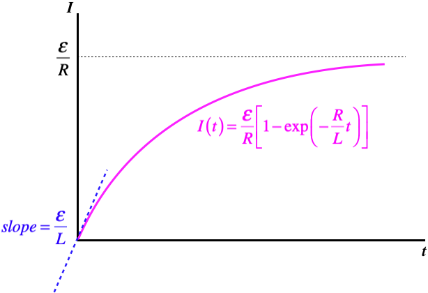
Let's check the extreme ends of this curve, to see if it makes sense. When the switch is first closed, the current grows at its greatest rate, but this is not infinity. That is, the current doesn't immediately jump to the value given by Ohm's law. The greater the inductance, the slower the initial growth in current is, since the slope of the current curve at \(t=0\) is inversely-proportional to \(L\). After a long time, the current-vs.-time curve flattens-out, and when the slope is zero, there is no emf induced in the inductor, which means that the current reaches the Ohm's law value – it gets to this point asymptotically.
Note that we can also witness this process in reverse – a circuit with an established current from which the battery is suddenly removed. In this case, we simply remove the \(\mathcal E\) term from the differential equation, and the result is exponential decay, like a discharging capacitor. The time constant for this case is the same as the case of growing current:
\[I\left(t\right) = I_oe^{-\frac{t}{\tau}}\;,\;\;\;\;\; \tau\equiv \dfrac{L}{R}\]
In terms of energy, it is easy to see what is going on here. The energy stored in the magnetic field is gradually converted into thermal energy energy by the resistor.
LC Circuits
Let's see what happens when we pair an inductor with a capacitor.
Figure 5.4.3 – An LC Circuit
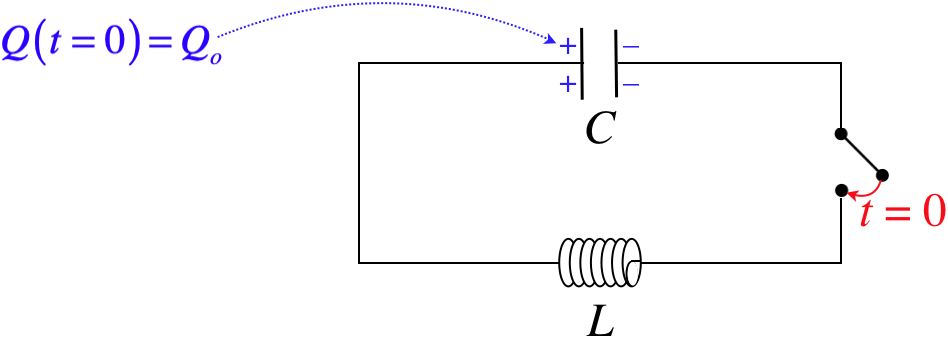
Choosing the direction of the current through the inductor to be left-to-right, and the loop direction counterclockwise, we have:
\[+\dfrac{Q}{C} -L\dfrac{dI}{dt}=0\]
Next we have to recall how to relate the charge on the capacitor to the current. When this current is positive, charge is leaving the capacitor, which means that a decrease in \(Q\) is related to a positive value of \(I\) according to:
\[I=-\dfrac{dQ}{dt} \]
Putting this in above gives the differential equation:
\[\dfrac{d^2Q}{dt^2} + \dfrac{1}{LC}Q = 0\]
This is another differential equation we have seen before, though it was not in this class. Yes, this is the same differential equation that comes about for a mass oscillating on a spring. The solution for \(Q\left(t\right)\) needs to be sinusoidal, since two derivatives of a sine or cosine function gives back a negative of itself (multiplied by a constant that comes from the chain rule). The solution to this particular case (with the starting charge at \(t=0\) given) is:
\[Q\left(t\right) = Q_o\cos\left(\omega t\right)\;,\;\;\;\;\;\omega\equiv \dfrac{1}{\sqrt{LC}}\]
Interpreting this result, we see that the charge actually sloshes back-and-forth between the plates (the charges on the plates actually eventually swap places!). We can also write down the equation for the current:
\[I\left(t\right) = -\dfrac{dQ}{dt} = Q_o\omega\sin\left(\omega t\right)=\dfrac{Q_o}{\sqrt{LC}}\sin\left(\omega t\right) = I_{max}\sin\left(\omega t\right)\;,\;\;\;\;\;I_{max}\equiv\dfrac{Q_o}{\sqrt{LC}}\]
We see that the current starts at zero, and grows to a maximum value, and this maximum occurs when the value of the sine is 1, which is the same time that the charge on the capacitor reaches zero. This actually gives us insight into the energy considerations for this circuit. Energy isn’t being converted to thermal energy by a resistor, so it has no way to exit, which means that the oscillations continue indefinitely. We know exactly how much energy the circuit starts with:
\[U_{tot}=\dfrac{Q_o^2}{2C}\]
When all of the charge is gone, the current hits a maximum, which means that all of the energy is then in the magnetic field. It’s easy to confirm that the energy is conserved:
\[U_{tot} = \frac{1}{2}LI_{max}^2 = \frac{1}{2}L\left(\dfrac{Q_o}{\sqrt{LC}}\right)^2 = \dfrac{Q_o^2}{2C}\]
Example \(\PageIndex{1}\)
Show that the total energy in the LC circuit remains unchanged at all times, not just when all the energy is in the capacitor or inductor.
- Solution
-
The energy stored in the system at a time \(t\) is the sum of the energies stored in each device:
\[U\left(t\right) = \frac{1}{2C}\left[Q\left(t\right)\right]^2 + \frac{1}{2}L\left[I\left(t\right)\right]^2 = \frac{1}{2C}\left[Q_o\cos\left(\omega t\right)\right]^2 + \frac{1}{2}L\left[I_{max}\sin\left(\omega t\right)\right]^2 \nonumber\]
We have already established that the maximum values are equal, so:
\[\frac{1}{2}LI_{max}^2 = \dfrac{Q_0^2}{2C}\;\;\;\Rightarrow\;\;\; U\left(t\right) = \dfrac{Q_0^2}{2C}\left[\cos^2\left(\omega t\right)+\sin^2\left(\omega t\right)\right] = \dfrac{Q_0^2}{2C}\nonumber\]
LRC Circuits
All that remains to examine in terms of circuits that combine different components is to put all of them together. We can guess the result – the resistance results in decay, as the energy in the circuit gets converted to thermal. The capacitance and inductance do their dance of oscillation between electric and magnetic field energy. Putting them all together results in the equivalent of a damped oscillator (a harmonic oscillator with friction).
Figure 5.4.4 – An LRC Circuit
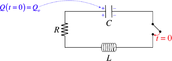
To get to this result, we (as usual) start with Kirchhoff's loop rule. This time the solution to differential equation has different characteristics, depending upon the values of the constants involved. For example, if the resistance is above a certain amount, the current dissipates before the charge is able to switch plates on the capacitor – it just decays directly down to zero. This is called an overdamped system. If the resistance is just barely large enough to cause this behavior, the system is said to be critically-damped. And if the resistance is low enough to allow oscillation, it is called under-damped. In this case, the charge does oscillate between the two capacitor plates, filling them a little less with every iteration.
Figure 5.4.5 – Current Behavior Based on Circuit Details
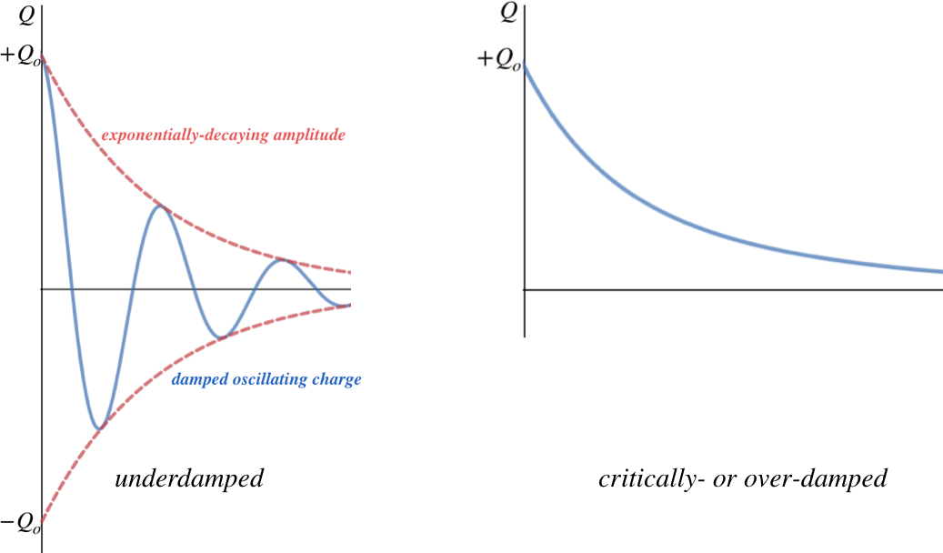
The critical criterion for determining which of these occurs is a comparison of \(R^2\) and \(\dfrac{4L}{C}\):
\[\begin{array}{l} \text{underdamped:} && R^2<\dfrac{4L}{C} \\ \text{critically-damped:} && R^2=\dfrac{4L}{C} \\ \text{overdamped:} && R^2>\dfrac{4L}{C} \end{array}\]