2.6: Additional Twists - Constraints

Let's Spice Things Up!

If Newton's laws are the main ingredients of the mechanics recipes we have been cooking-up, then the time has come to add the spices. Actual physical systems are typically characterized by more than just the three laws of motion. Very often there are other restrictions – called constraints – that relate physical quantities to each other. Some of these are independent of Newton's laws of motion, while others are "rules of thumb" that ultimately come from Newton's laws.

We have actually seen a couple of examples of these already, in the examples we look at in the previous section, though we never referred to them in this way. One of them is the relationship between the kinetic friction force and the normal force for two surfaces. This relationship (equation) does not come from the invocation of Newton's second or third law, it is just an extra equation that we can use to solve problems that include the feature of rough surfaces sliding across each other. Another example we have seen is the formula for centripetal acceleration. Newton's second law tells us how to relate forces to accelerations, but this specific relationship between acceleration and velocity for the case of circular motion only applies to special cases.

We will add to our "spice rack" of possible constraints in this section, and in so doing, we will greatly multiply the variety of mechanics problems we can solve.

Constraints on Forces

The two quantities in Newton's second law that can be constrained are force and acceleration. We will look at each possibility in turn, starting with force constraints.

Pulleys

One of the favorite devices for physics mechanics problems is the pulley. As usual, we will start with the simplest model, which in this case means we will assume that pulleys are massless and frictionless. As we will see more clearly later in the course, these two conditions are sufficient to ensure that the tension applied at one end of the rope is the same as the tension applied at the other, even though the intermediate section of the rope goes around one or more pulleys. This means the measured tension force can have different directions, depending upon where it is measured, but it always has the same magnitude. This is a constraint on the tension forces present in a physical system.

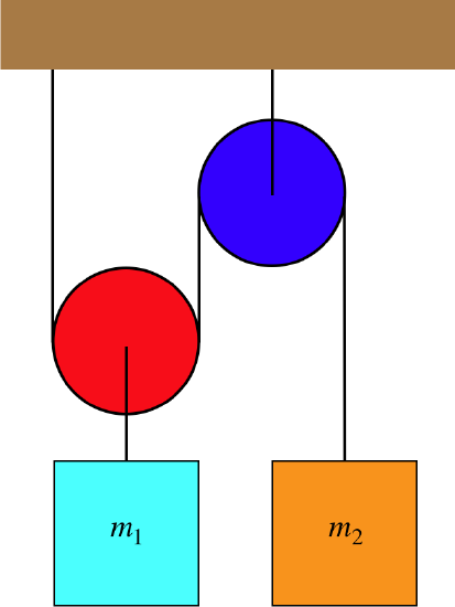
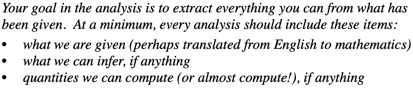
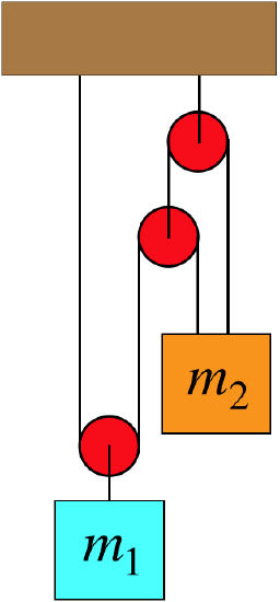
Pulleys get especially interesting in situations like the following example, where at least one of the pulleys is able to move. The two blocks remain at rest in the system of ropes and pulleys shown in the diagram. Given this information, can you conclude how the two masses compare?

Figure 2.6.1 – Blocks Hanging from Multiple Pulleys

By now we know that when it comes to analyzing the forces present in a system, there is no better tool than the free-body diagram. We begin there:

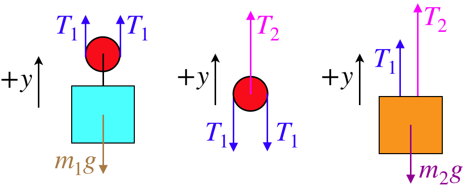
Figure 2.6.2 – Free-Body Diagrams of Blocks and Pulleys

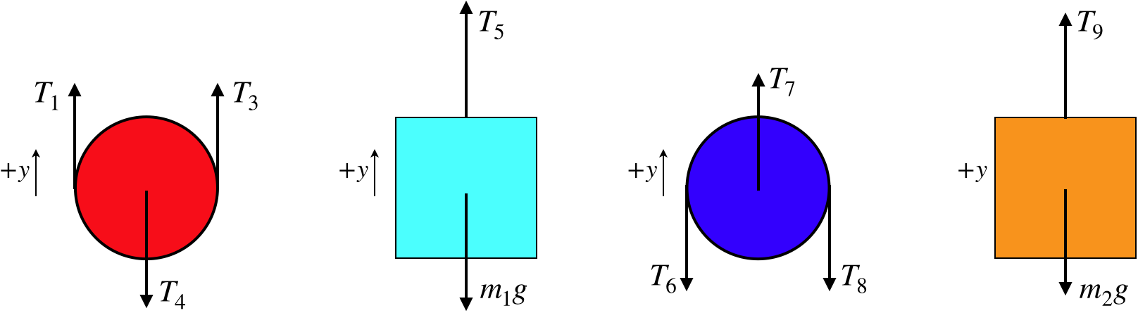
Look at all those tension force vectors! There is one for every segment of rope pulling on an object. One might ask why there are two tension force vectors drawn for the same rope on each pulley. The simplest answer is to consider what you would feel if you grabbed the rope on both sides of the red pulley, and cut the rope above the two points where you are holding. Clearly you would feel the pulley pulling down on both ends of the rope. If you feel forces down by each end of the rope, then the pulley must feel forces up by each end as well, according to Newton's third law.

Here is where our pulley force constraint comes into play. Assuming the pulleys have negligible mass (or are static, and these are both), and assuming their axles are frictionless, then we can use the constraint that tension forces exerted by every segment of a single continuous piece of rope has the same magnitude. There are three ropes involved here, so this constraint in mathematical terms gives:

\[T_1=T_3=T_6=T_8=T_9\;,\;\;\;\;T_4=T_5\]

Alert

We must be careful not to equate too many of these tensions – this constraint only holds for a single, continuous piece of rope.

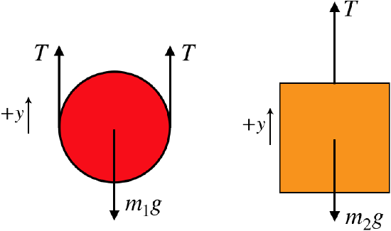
This constraint, if used carefully (i.e. making certain that the conditions required are in place), allows us to greatly streamline our problem-solving process. For example, when drawing the FBDs, we can avoid 9 different tension force labels, and just label all the tensions from the long, common rope simply "\(T\)." Another simplification for this diagram is noting that if we put the (red) pulley that is free to move up and down into a single system with the (blue) block that moves with it, then we can ignore the internal tension force (\(T_4=T_5\)) altogether, and just label the downward force with the weight of the block. Let's incorporate these shortcuts into a revised FBD before proceding with our analysis. If we note that the FBD of the blue pulley is of no value to our analysis, we get the following very efficient FBDs:

Figure 2.6.3 – Streamlined Free-Body Diagrams of Blocks and Pulleys

The next step in our analysis is to sum the forces for each object and apply Newton's second law, which in this case involves zero acceleration. In taking the sum of forces, we have to take care to correctly use our coordinate system:

\[ \left. \begin{array}{l} 0 = a_1 = \dfrac{F_{net \; 1}}{m_1} = \dfrac{2T - m_1 g}{m_1} \;\;\; \Rightarrow \;\;\; T = \dfrac{m_1 g}{2} \\ 0 = a_2 = \dfrac{F_{net \; 2}}{m_2} = \dfrac{T - m_2 g}{m_2} \;\;\;\; \Rightarrow \;\;\; T = m_2 g \\ \end{array} \right\} \;\;\; \Rightarrow \;\;\; m_1 = 2 m_2\]

Notice that the light weight \(m_2\) holds up the heavier one because the placement of the pulley allows us to use the tension from the same rope twice on the heavier mass. This trick can actually be repeated as many times as we like (the pulley can have multiple tracks in it), and this enables us to lift very heavy weights with very little force. This invention is called a block and tackle. They are used for sailing ships (the heavy sails and boom can be pulled tighter), lifting engine blocks, and many other applications.

Analyze This

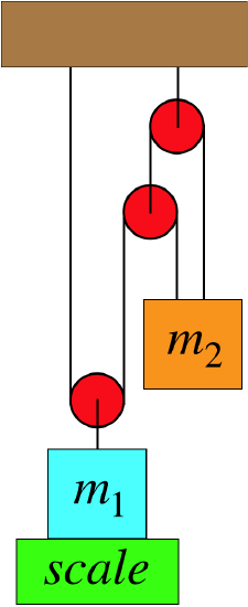
In the system shown below, the blue block remains at rest on the scale while it is attached to the pulley system as shown. All of the pulleys are massless and frictionless, and the rope is massless.

Analysis

As usual, the first step in analyzing such systems is to draw a FBD. In this case, we will employ whatever "shortcuts" indicated above that we can, but we need to be extra careful when multiple ropes are involved!

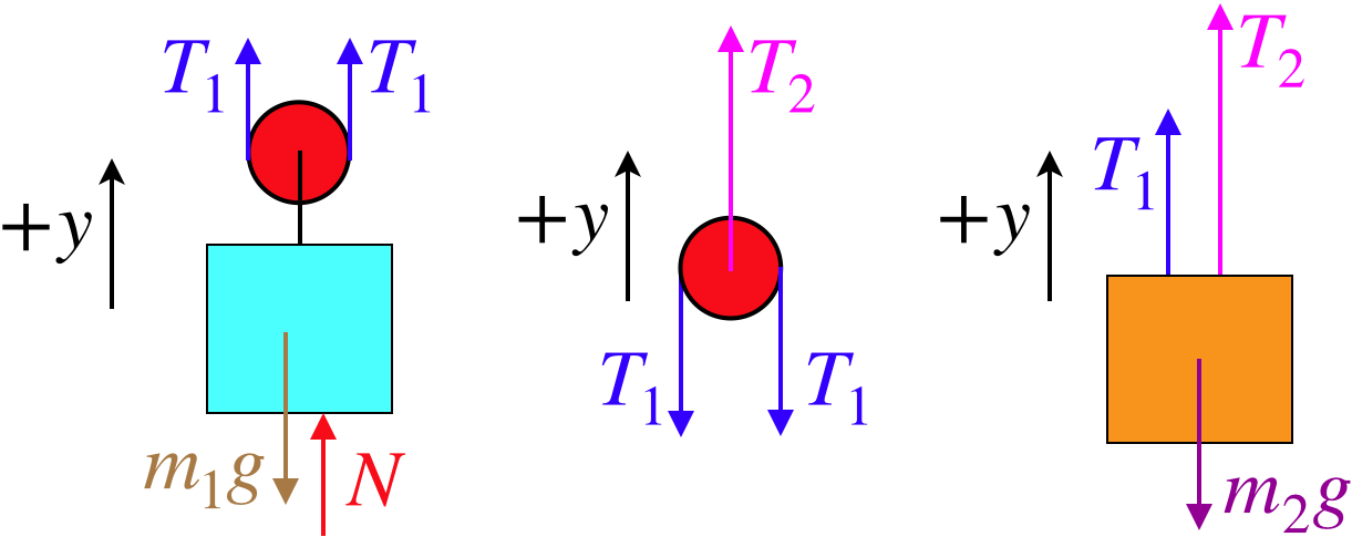
As noted in the text above, a FBD of the fixed (highest) pulley provides no useful information, since it only introduces the force by the ceiling pulling it up. If we are asked about this force, then we would have to add this FBD to the collection. For these three FBDs, we can construct the equations that result from Newton's second law, with zero acceleration:

\[F_{\text{net}}=+2T_1+N-m_1g=0\;,\;\;\;\;F_{\text{net}}=T_2-2T_1=0\;,\;\;\;\;F_{\text{net}}=+T_1+T_2-m_2g=0\nonumber\]

We can now (for example) eliminate the variables \(T_1\) and \(T_2\) from the equations and get the scale reading (the normal force) in terms of the blocks' masses:

\[T_2=2T_1\;\;\;\Rightarrow\;\;\;2T_1=\frac{2}{3}m_2g\;\;\;\Rightarrow\;\;\;N=\left(m_1-\frac{2}{3}m_2\right)g\nonumber\]

It makes sense that the heavier \(m_2\) is, the less force will be registered by the scale, since the orange block is pulling up on the blue block through the pulley system.

Friction

Another constraint on forces is one we have discussed previously – how the friction force between surfaces is related to the normal force between those surfaces. While the friction and normal forces appear in the equations that come from Newton's second law, the relationship between friction and normal force is "extra." We have already seen examples of this in action for kinetic friction in the previous section, so here we will direct our attention to the constraint for static friction.

When one has a system of equations, and then throws in an additional equation like \(f_k=\mu_kN\), it is easy to incorporate into the algebra. Incorporating an inequality like \(f_s\le\mu_sN\) is tougher, mainly because there is a conceptual element to it. Generally it shows itself in the statement of the question with language like, "Find the largest (or smallest) force for which...", or "Find the value of <whatever> at which the system starts to move".  That is, there needs to be some mention of an extremum. This is because the extremum will trace its roots back to the maximum value of static friction, and when we are interested in the maximum value, our inequality becomes an algebraically-useful equality.

Analyze This

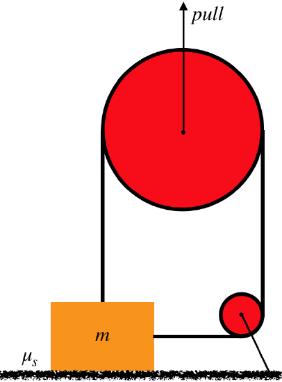
A rope is fastened to a block in two places and passes through a system of two massless, frictionless pulleys, as shown in the diagram below. The block rests on a rough horizontal surface. The bigger pulley can be pulled upward.

Analysis

Start with the free-body diagrams and coordinate systems. The FBD of the smaller pulley will yield us nothing useful, so there are just two FBDs to draw. Note that the tension on the side of the block comes from the same rope as the tension on the top of the block, so thanks to the pulley constraint, they are equal, and we'll label them both the same "\(T\)".

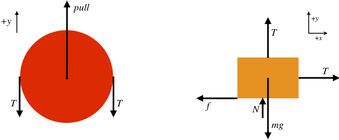
The block is not accelerating at all (nor is the pulley), so the sum of the forces in each of the \(x\) and \(y\) directions comes out to zero.

\[F_{\text{net}}=+pull-2T=0;,\;\;\;\;F_{\text{net }x}=+T-f_s=0\;,\;\;\;\;F_{\text{net }y}=+T+N-mg=0\nonumber\]

Obviously if we pull up with sufficient force, then we'll lift the block off the horizontal surface. In particular, to lift the block the FBD of the block shows that the tension force pulling up needs to exceed the weight of the block. With two such tension forces pulling down on the pulley, we would have to pull up on the pulley with twice the weight of the block to get it to accelerate vertically. But the interesting part of this system lies with the horizontal motion...

As long as this system remains static, the friction force will only react to the other forces to hold the block in place horizontally. We can't say anything about this force without more information, but it is natural to ask, "How hard to we have to pull up on the larger pulley in order to get the block to start moving? We would expect that the force required is less than the force needed to left the block, computed above, but how do we find this force?

If we have to pull "just hard enough" to get the block moving, then this occurs when the horizontal pull equals the maximum static friction force, which converts our static friction inequality into a constraint equation:

\[ f = \mu_s N\nonumber\]

Note that the block will have to start sliding before it starts rising, because rising requires than the normal force goes to zero, and it will slide when the static friction force is small-but-non-zero. Now solve the equations simultaneously to get:

\[ T= \mu_s N=\mu_s\left(mg-T\right)\;\;\;\Rightarrow\;\;\;pull=2T=\dfrac{2\mu_s}{1+\mu_s}mg\nonumber \]

Constraints on Acceleration

We now turn our attention to constraints on acceleration. These are "constraints" in a more literal sense than for forces, in that they are not shortcuts for more complicated cases. Acceleration constraints are purely mathematical (not physical) relationships, and therefore require fewer – if any – special conditions. These constraints on acceleration come in several varieties – from restrictions between components of acceleration for a single object, to accelerations of separate (connected) objects, to restrictions due to "special" motion.

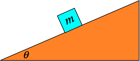
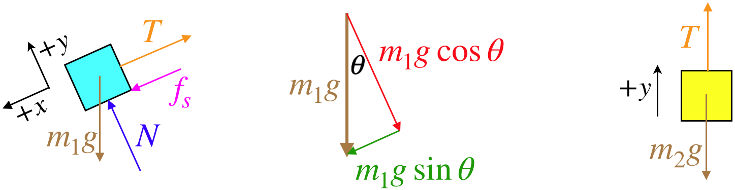
Inclined Planes

In a large percentage of our examples so far, objects have been accelerating either horizontally or vertically. These have actually been "constraints" of a sort, because we know that when an object is accelerating along a horizontal surface (i.e. the object is "constrained to remain on the horizontal surface"), then we can immediately infer that its vertical acceleration is zero, and we can then plug this fact into the vertical equations for Newton's second law.

But now let's suppose that the object is confined to travel along a different surface. We will eventually talk about confinement to curved surfaces, but the simplest "new" case is a flat surface that makes an angle with the horizontal – a so-called inclined plane. This constraint forces the horizontal and vertical components of acceleration to have a specific relationship with each other. Namely, if the angle the plane makes with the horizontal is \(\theta\), then \(\dfrac{a_y}{a_x}=\tan\theta\). So if we sum our forces along the horizontal (\(x\)) and vertical (\(y\)) axes, and apply Newton's second law, then we have an additional equation to throw into the mix thanks to the constraint that the object remains in contact with the inclined plane. To see this in action, let's look at the simplest possible case – a block on a frictionless inclined plane:

Figure 2.6.4 – Block on a Frictionless Inclined Plane

With no friction present, there are only two forces on the block. Drawing the free-body diagram and resolving the angled normal force into the usual horizontal and vertical components gives:

Figure 2.6.5 – FBD of Block on a Frictionless Inclined Plane

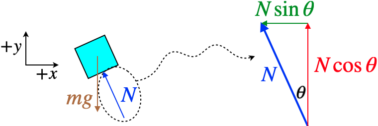
[The reader is encouraged to do the geometry to confirm that the angle \(\theta\) in the normal force resolution is the same as the angle of the inclined plane up from the horizontal.]

Now we apply Newton's second law to this diagram, for both components of the net force:

\[F_{\text{net }x}=-N\sin\theta=ma_x\;,\;\;\;\;F_{\text{net }y}=N\cos\theta-mg=ma_y\]

Now we can do a bit of algebra, and apply our acceleration component constraint to get (after some trig identities):

\[-\dfrac{N\cos\theta}{N\sin\theta}=\dfrac{ma_y+mg}{ma_x}\;\;\;\Rightarrow\;\;\;-\cot\theta=\tan\theta+\dfrac{g}{a_x}\;\;\;\Rightarrow\;\;\;a_x=-g\sin\theta\cos\theta\;\;\;\Rightarrow\;\;\;a_y=a_x\tan\theta=-g\sin^2\theta\]

The negative signs have appeared because the coordinate system chosen has to-the-right and upward as the positive directions, and this block accelerates to-the-left and down. We are interested in the motion of the block, which means its total acceleration along the inclined plane. We can get this from the components of acceleration:

\[a=\sqrt{a_x^2+a_y^2}=\sqrt{g^2\sin^2\theta\left(\cos^2\theta+\sin^2\theta\right)}=g\sin\theta\]

It turns out that we can save ourselves some of the algebra above when it comes to inclined planes by using a common trick. We have been treating our horizontal/vertical \(x\), \(y\) coordinate system like it is sacred, but it is certainly not. We can choose any axes we like, as long as we stick with them throughout, and correctly reference the forces on those axes. Consider what happens if we choose the following coordinate system:

Figure 2.6.6 – Useful Coordinate System for an Inclined Plane

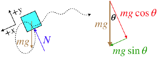
We have the same physical situation – same FBD – but this time the normal force is parallel to the \(y\)-axis, and it is the gravity force that we have to break into components. So what have we gained? The block is constrained to slide along the surface, so it only accelerates parallel to the \(x\)-axis. This makes the equations from Newton's second law easier to work with, giving the same answer as above for the acceleration immediately:

\[F_{\text{net }x}=mg\sin\theta=ma_x=ma\;\;\;\Rightarrow\;\;\;a=g\sin\theta\;,\;\;\;\;F_{\text{net }y}=N-mg\cos\theta=ma_y=0\]

This coordinate system choice is appreciated even more when one encounters a problem with other forces that are also parallel to the rotated axes (like friction, parallel to the surface). The fewer forces that need to be broken into components, the better.

Analyze This

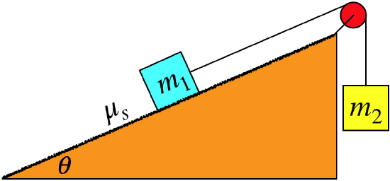
The system shown in the diagram below remains at rest. The rope and pulley are massless, and the pulley is frictionless, but the inclined plane is not.

Analysis

There is obviously a lot going on here, but as always, our analysis just needs to take it one step at a time. We start as usual with free-body diagrams, but the FBD of the blue block poses a bit of a puzzle for us. With a component of the gravity force acting down the plane, and the tension force acting up the plane, we can't tell from looking at the diagram which of these two forces is greater. The static friction force only reacts to the other forces, so if the tension force is greater, then the friction force must point down the plane to keep the block from sliding up, and if the tension force is less, then the friction force points up the plane to keep the block from sliding down. (The friction force could even equal zero, if the magnitude of the tension force happens to be equal to \(m_1g\sin\theta\).)

The answer to this conundrum is this: As an unknown, the static friction force must point either in the \(+x\) or \(–x\) direction. If we happen to draw the vector in the wrong direction, then after we do the math to obtain an answer for this force, then the answer will have the right magnitude, but will have a negative sign. This doesn't mean we have made a mistake – the FBD is there to help us solve the problem, which it did! It allowed us to compute the magnitude, and with the sign, it also told us the direction. So just draw the friction force on the FBD in either direction – it is a means to an end, not a declaration of which way you believe the direction to truly be.

Now for Newton's second law. With the system remaining at rest, we can immediately plug-in zero for the accelerations:

\[F_{\text{net }x}=+m_1g\sin\theta+f_s-T=0\;,\;\;\;\;F_{\text{net }y}=+N-m_1g\cos\theta=0\;,\;\;\;\;F_{\text{net}}=+T-m_2g=0\nonumber\]

We can go no further without more information, which (for example) could trigger something like the static friction / normal force equation of constraint.

Pulleys

Another way that accelerations can be constrained involves ropes moving through pulleys. This constraint relates the motion of one object to that of another when they are connected through a system of pulleys. The only assumption required for this kind of constraint is that the rope does not stretch – however much it gets shorter in one segment, it gets longer by the same amount in another segment. Let us return to the system shown in Figure 2.6.1 and ask the following question: If the block \(m_1\) rises a distance \(\Delta y \), what happens to the block \(m_2\)?

First of all, it should be clear that \(m_2\) drops as \(m_1\) rises, so the only question is, how far? This may not be apparent at first, but think of it this way: When the pulley holding \(m_1\) moves up 1 unit of distance, both segments of rope going up from that pulley get shorter by 1 unit. These two units of rope don't simply vanish, and in fact they are taken-up by the free end of the string, which is attached to \(m_2\). This means that as \(m_1\) rises a distance of \(\Delta y \), \(m_2\) must drop exactly twice that far: \(2\Delta y\).

What does this say about the comparison of the speeds and accelerations of the two blocks? Well, they are required to move simultaneously, so every unit of length that \(m_1\) rises is matched by a drop of \(m_2\) that is twice as much, which means that \(m_2\) always moves at twice the speed and accelerates twice as much as \(m_1\). If this system is not balanced (as it was in the original example), then applying Newton's second law to both blocks includes two accelerations, but these are constrained to be related to each other by a factor of two, providing us with an additional constraint equation:

\[ 2\left| a_1 \right| = \left| a_2 \right|\]

What's with the absolute values, you ask? Well, these variables can have positive or negative values, and we must be careful when it comes to signs. In particular, we have to look at how our constraint relates to our choice of coordinate systems for the two blocks. In Figure 2.6.2, we chose "up" as the positive direction for both blocks. So we need to ask ourselves, "If one block experiences a positive displacement, what is the sign of the displacement of the other block?" In this case it's clear that the displacement of the two blocks have opposite signs. Therefore the constraint equation for the block accelerations is:

\[ 2a_1 = -a_2\]

Note that it is perfectly fine to set up different coordinate systems for the two blocks – each FBD is entitled to its own individual coordinate system. How the coordinate systems relate to each other affects the equation of constraint. So for example, if we had instead chosen downward to be the +\(y\)-direction for block #2 (but left upward as positive for the other block), then there would be no need for the minus sign in the constraint equation – positive displacements of one block correspond to positive displacements of the other block. We see that there is therefore no "correct" choice of coordinate system, but we must take care when the time comes to combine the equations from the two FBDs, to ensure that the constraint equations relate the variables correctly.

With this constraint mechanism in mind, let's recycle a pulley system we analyzed above, this time without the condition that it remains static with the blue block resting on a scale:

Analyze This

In the system shown below, the blocks are free to accelerate. All of the pulleys are massless and frictionless, and the rope is massless.

Analysis

[The analysis of this system teaches us a very important lesson about these types of problems: Even though this will clearly behave very differently from the case studied above, much of the early analysis is the same. This demonstrates why it is important to practice the little pieces of analysis, as they come up over and over.]

The FBDs for this system are the same as those above, with the exception of the normal force coming from the scale:

Okay, now we invoke Newton's second law. Unlike the previous case, we need to include non-zero accelerations:

\[F_{\text{net}}=+2T_1-m_1g=m_1a_1\;,\;\;\;\;F_{\text{net}}=T_2-2T_1=m_{pulley}a_{pulley}\;,\;\;\;\;F_{\text{net}}=+T_1+T_2-m_2g=m_2a_2\nonumber\]

Okay, now is where things get a bit different. First, we note that the equation of motion for the pulley includes the mass of the pulley, which we are given is zero. So the relationship between the two tensions is the same as before:

\[T_2=2T_1\nonumber\]

And now the time has come to relate the constrained accelerations of the two blocks. [This is quite tricky – much trickier than you will encounter on your own in this class, but we'll slog through it in the hope that it helps you to do simpler examples on your own.] Start by defining the positions of the three moving objects, measured as the distance down from the highest pulley: \(y_1\), \(y_p\), and \(y_2\). The lengths of the long and short ropes (\(L\) and \(l\), respectively) can be written in terms of these distances (plus a constant to account for the radii of the pulleys and in the case of the longer rope, the distance of the highest pulley from the ceiling):

\[\begin{array}{l} L=const+\text{left segment}+ \text{middle segment}+\text{right segment} =  const+y_1+\left(y_1-y_p\right)+\left(y_2-y_p\right)=const + 2y_1-2y_p+y_2\\l=const+\text{left segment}+\text{right segment} =  const+y_p+y_2\end{array}\nonumber\]

We are interested in how the change in the height of the blue block is related to the change in height of the orange block, which means we are looking to relate \(dy_1\) to \(dy_2\). The length of the rope doesn't change, nor does the constant, so:

\[dL=0=0+2dy_1-2dy_p+dy_2\;,\;\;\;\;dl=0=0+dy_p+dy_2\;\;\;\Rightarrow\;\;\;dy_1=-\frac{3}{2}dy_2\nonumber\]

From this result, we conclude that the magnitude of the acceleration of the blue block is 1.5 times the acceleration of the orange block. Notice that we have chosen 'up' to the be positive direction for both blocks, but when one block goes down, the other must go up. So the accelerations must have opposite signs, and we conclude:

\[a_1=-\frac{3}{2}a_2\nonumber\]

From this and in equations above, one can compute the accelerations of the blocks in terms of their masses. Sparing the reader the algebra, it comes out to be:

\[a_1=\frac{6m_2-9m_1}{9m_1+4m_2}g\;,\;\;\;\;a_2=\frac{6m_1-4m_2}{9m_1+4m_2}g\nonumber\]

The tensions in the two ropes can also be computed in terms of the two masses:

\[T_1=\frac{5m_1m_2}{9m_1+4m_2}g\;,\;\;\;\;T_2=\frac{10m_1m_2}{9m_1+4m_2}g\nonumber\]

Circular Motion

The last of the accelerated constraints involves knowing something specific about the acceleration of the one or more objects involved. A trivial case would be that you could be simply given the acceleration. Another possibility is that the object could be moving in a straight line and you could be given details about its motion (initial speed, distance traveled, etc.), and the acceleration could be computed using kinematics. But the most interesting and useful ways to constrain the acceleration of an object is to have it move in a circle, so that it experiences a centripetal acceleration.

Conceptual Question

Everyone knows that a spring can only be stretched if it is pulled from both ends – pulling from one end only moves the whole spring without stretching it. With this in mind, consider the following: A block is attached to one end of a massless spring, the other end of which is attached to a vertical fixed peg in a frictionless horizontal surface. The block is spun around a circle, and the spring stretches as a result of this motion, (which means that both ends are being pulled). In fact, the faster the motion, the more the spring stretches. Clearly the peg is pulling on one end of the spring as the block goes in the circle, but what force is pulling the block outward to stretch the spring?

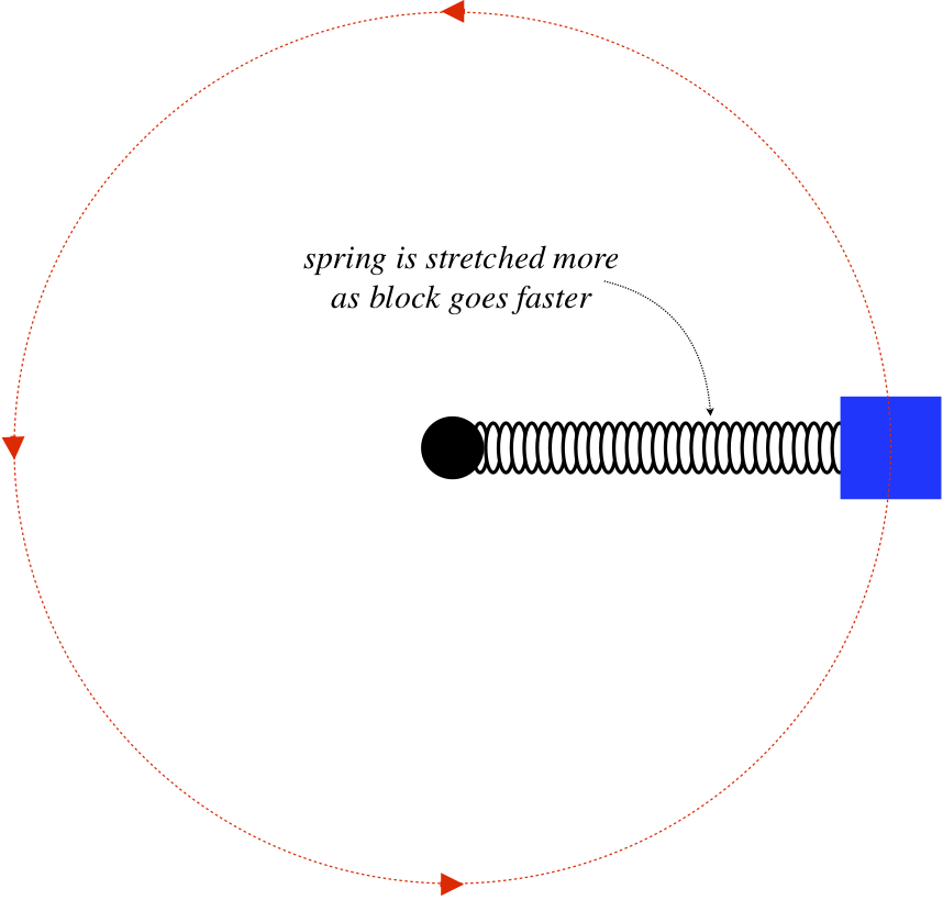
Solution

The block is not pulled outward! It is only pulled inward (by the spring). It is not the block that needs to be pulled outward to stretch the spring, but rather the spring that needs to be pulled that way. The spring pulls the block inward (keeping it accelerating centripetally), and the third-law-pair force of the block on the spring is what pulls the spring outward. This is a fantastic example of how imprecise wording can get someone in trouble in physics discussions.

This points out possibly better than any other example the importance of isolating objects with force diagrams. The block here is not a conduit for some mysterious force pulling out on the spring – it is the object pulling out on the spring. You thoroughly need to trust the third law here to get the force between the spring and the block, and you need to thoroughly trust the second law to realize that the block does not require another force on it outward to balance the spring force, because it is accelerating.

Now for an example that incorporates circular motion. What makes this problem interesting is the information that is hidden within the wording...

Analyze This

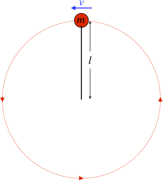
A rock on a string flies around (with negligible air drag) in a circle in a vertical plane (in the presence of the earth's gravity) such that it just barely gets by the top (the string remains at its full length at the top of the circle, just barely not going limp) as it continues in its circular path.

Analysis

Start with a free-body diagram. Clearly there is gravity acting on the rock, so the only question is whether the string is contributing a tension force. While it is straight, we are told that the rock "barely gets by the top", which means that the string has gone limp at the peak, and the tension force is zero. That makes the FBD rather simple:

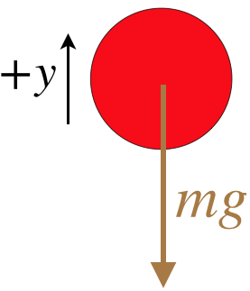
Though we have not stated so explicitly, we can think of the "tension force from string equals zero" as a force constraint. It is information given to us (in an obscure manner) that pertains to the value of one of the forces that is not derived from the application of Newton's laws, so it fits the description perfectly. Whether we call it a constraint or not isn't important – what matters is that we can extract this piece of physical data from the information given.

Next we turn to the acceleration constraint – the rock is traveling in a circle. If we call the speed of the rock at the top of the circle "\(v\)," and the length of the string "\(l\)," as indicated in the diagram, then  the centripetal acceleration toward the other end of the string is:

\[a_c=\dfrac{v^2}{l}\nonumber\]

Relating this acceleration to the only force present, we see that these vectors are in the same direction, as they should be, and Newton's law gives us a result that expresses the velocity of the rock in terms of only the length of the string!

\[F_{\text{net}}=ma\;\;\;\Rightarrow\;\;\; mg=ma_c=m\dfrac{v^2}{l}\;\;\;\Rightarrow\;\;\;v=\sqrt{gl}\nonumber\]