5.3: Fluid Flow

Steady-State Systems

In the Energy-Interaction model, the change in energy (or other state variables) was always from an initial to final state; that is, from a state earlier in time to a state later in time. The interaction of interest occurred during the time between the initial and final states. Now we will look at a steady-state energy model where the states are not distinguished in time; rather they are distinguished by spatial location in the physical system.

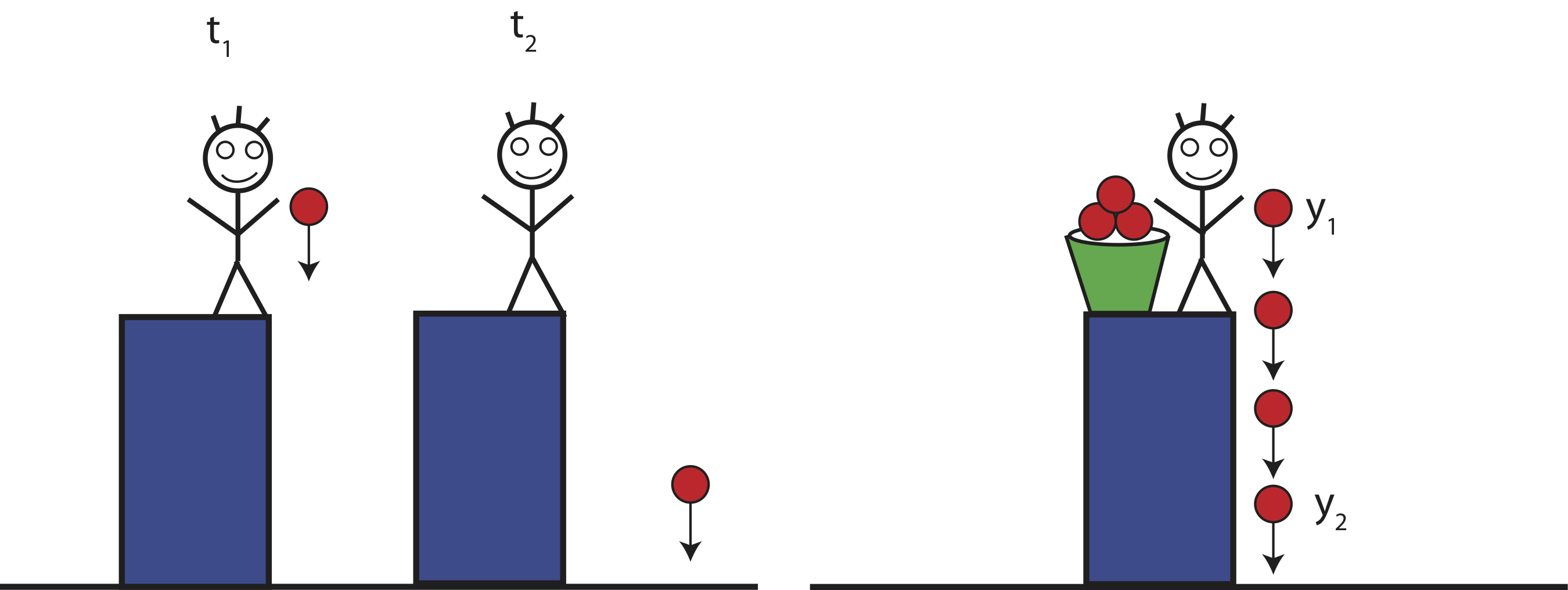
When we studied systems in 7A we analyzed how energy changed as a function of time during some interaction. In Figure 5.3.1 shown below, a person drops a ball at some initial time, \(t_1\). We can apply conservation of energy to figure out how the energy of the ball at some later time \(t_2\) changed. In a different scenario, instead of dropping one ball the person drops multiple balls at equal time intervals, such as in the drawing on the right in Figure 5.3.1. In this case the system of falling balls looks identical as a function of time. If you took a picture of the left scenario at \(t_1\) and then later at \(t_2\), you would see the ball higher and then lower, respectively. This this system is changing with time. On the other hand, if you took two pictures of the right scenario at two different times, the pictures would look identical, if the balls are indistinguishable, even though the balls are moving. We call this scenario a steady-state system. For a steady-state system instead of analyzing energy differences between two time periods, such as \(t_1\) and \(t_2\) in the left diagram, we will analyze energy differences between two spatial locations, such as \(y_1\) and \(y_2\) in the right diagram below.

Figure 5.3.1: Time Varying versus a Steady-State System.

Flow Rate and Continuity

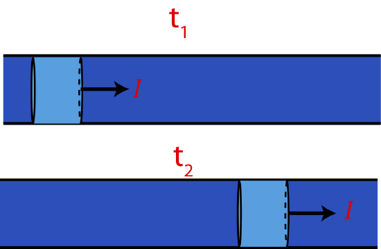
A flowing fluid at equilibrium is an example of a steady-state system. If you are observing a steady-state fluid system flowing past you, the system looks identical with passage of time. For the fluid to be in a steady-state, it cannot pile up or leak out of anywhere (what goes in at one end of the pipe must come out at the other end). In other words, the amount of time that it takes for a volume of fluid to flow past one point must equal the amount of time it takes for that same volume to flow past another point at a later time. As depicted in Figure 5.3.2 this means that the light blue fluid element at some initial time \(t_1\) will have the same flow rate as at a late time \(t_2\). 

Figure 5.3.2: Steady-State Fluid Flow System.

We define the rate at which the fluid flows, the volume of fluid passing through the pipe at a particular location along the pipe per second, the volumetric flow rate, \(I\), sometimes referred to as current:

\[I=\dfrac{dV}{dt}\label{flow-rate}\]

with standard SI units of \(m^3/s\). The letter \(“I”\) is a standard symbol for electric current, so we will use it here in our discussion of fluids as the symbol for the volumetric flow rate or current since our next discussion will be on electric flow systems. In everyday language we do often refer to volumetric flow rate as "current", such as "this river has a fast current". (Advanced texts in other disciplines might use other symbols for flow rate, such as \(Q\), for example.)

When the fluid is in a steady-state and is incompressible (uniform density throughout), it cannot pile up or leak out. This means the current is conserved and remains constant in space throughout the entire fluid system. This is known as the continuity equation or conservation of mass:

\[I=\text{constant}\]

For this fluid dynamic model to work the flow has to be laminar. This means that neighboring fluid particles are flowing nearly parallel to each other, known as a streamline.  When the flow becomes too fast it the streamline becomes turbulent, resulting in swirls and non-linear and non-laminar flow. Thus, in our model we will confine ourselves to slower and linear flow rates.

For static fluids in equilibrium all locations in the connected fluid system with a constant density must have the same total energy-density. For flowing fluids, once steady-state has been reached, all locations in the connected fluid system must also have the same total energy-density if there are not external sources that either add or remove energy.  We will look at those cases shortly. We make the restrictions that the fluid is incompressible and that all elements of the fluid move uniformly at the same speed at any particular cross-section. We will now proceed to write down the energy-densities that are relevant for a steady-steady flowing fluid.

Kinetic energy-density

Let us think what happens in a fluid flowing through a pipe system where the pipe either narrows or widens. If the system is in a steady-state, the continuity equation tells us that current must be constant throughout the pipe system. Because we are dealing with an incompressible fluid that has fixed density, there is a simple relation between the velocity of the fluid and the cross-sectional area of the pipe. Figure 5.3.3 depicts a segment of a pipe where it becomes wider. 

Figure 5.3.3: Fluid Flow in a Non-uniform Pipe.

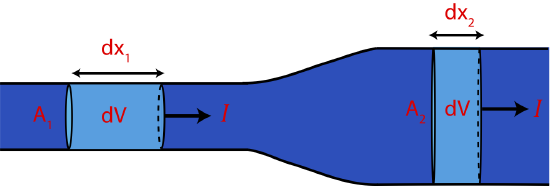
The same volume element, \(dV\), in the narrow part of pipe has to pass through the wider section of the pipe at the same rate.  We can rewrite the volume element, \(dV\), as the product of its cross-sectional area, \(A\) and the horizontal distance, \(dx\): \(dV=Adx\). The rate at which the fluid moves perpendicular to the pipe's cross-sectional area (or horizontally in Figure 5.3.3)  is defined as the fluid velocity, \(v=dx/dt\).  Thus, we can write Equation \ref{flow-rate} for flow rate as:

\[I=\dfrac{dV}{dt}=A\dfrac{dx}{dt}=Av\]

Applying the continuity equation, which states that current must remain the same in a steady-state fluid system, between the narrow and wide regions of the pipe system in Figure 5.3.3, we find that:

\[A_1v_1=A_2v_2\label{continuity}\]

The above result tells us that if the cross-sectional area changes, then the velocity of the fluid must change to keep the flow rate constant. The fluid speeds up when entering a narrower section and slows down when entering a wider segment of the pipe.

Alert

Although, the volumetric flow rate, or current, and the fluid velocity are both related to the rate at which the fluid moves, these quantities describe different fluid properties. Flow rate is the rate of volume per unit time and has units of, \(m^3/s\).  Fluid velocity is the rate at which the fluid moves on average in the direction perpendicular to the cross-sectional area of the container confining the fluid and has units of speed, \(m/s\). Fluid velocity describes average motion since each fluid particle is moving in random directions, but when averaged over all the particles there is a net "ordered" motion in the direction of the fluid velocity. Current and velocity are related to each other, since the greater current the greater the velocity.  However, once the fluid is in a steady-state the current which is determined by the properties of the entire system will stay constant throughout the fluid system from one location to another. The fluid velocity, on the other hand, will change if the cross-sectional area of the pipe changes.

The total energy \(E_{\text{total}}\) of the fluid element of volume \(dV\) will consist of the internal energy \(U\) (thermal plus all bond systems) plus any macroscopic energies. At first, we will neglect friction and assume that internal energy stays constant, which describes non-dissipative flow. As established in Equation \ref{continuity} the speed of the fluid will change when the pipe's cross-sectional area changes. Since speed is an indicator of kinetic energy this implies that a change in area will result in a change of translational kinetic energy-density, "density" since we describe fluids in terms of their "energy-density". We will omit in this treatment rotational motions, like the vortices that sometimes form when water goes down the drain of your bathtub, since in our model the flow is laminar.

Using the expression for translational kinetic energy \(KE=\frac{1}{2}mv^2\), dividing by volume to convert to an energy-density, and then using \(\rho=m/V\), we find that change in kinetic energy-density between two locations is given by:

\[ \frac{\Delta KE}{V}=\frac{1}{2}\rho\Delta (v^2)\]

Based on Equation \ref{continuity} the change in kinetic energy-density will be non-zero only when the pipe's cross-sectional area will change between the two points being analyzed. It is only the difference in the areas between the initial and final locations that will matter. For example, if a pipe gets wider in the middle of the interval analyzed but then returns to its original width at the end, the speed of the fluid will also return to its original value, and the kinetic energy will not change between the start and the end of the pipe.

In Section 5.2 we established how gravitational potential energy-density and pressure change with depth. For a dynamic fluid system we will typically ignore any height variations within a horizontal pipe since pipes are typically too narrow to result in any significant pressure changes even within a more dense liquid. However, if we are considering a pipe which is not positioned horizontally, such as water flowing downward from a reservoir at high elevation or from a water tower, or water flowing upward to the second floor of a house from a water tank on the ground floor, changes in gravitational energy-density need to be considered.

Combining  pressure and gravitational potential energy-density from Section 5.2 and kinetic energy-density terms, the conservation of energy-density equation becomes:

\[\Delta P+\rho g \Delta y + \dfrac{1}{2} \rho \Delta (v^2)= 0\label{standard-Bernoulli}\]

The equation above is often referred to as the Bernoulli equation.

Thermal energy-density

In many physical systems although friction is never completely absent, it is often negligible due to other dominating effects. For example, you can determine that a ball falling from a few meters conserves its mechanical energy to a great precision. Thus, in the case of the ball we can neglect the effects of air friction. This is no longer true for a piece of paper where its small weight and larger surface area make air friction a much greater effect.

Likewise, in some cases friction in fluid flow is negligible compared to other transfers of energy. The traditional Bernoulli Equation \ref{standard-Bernoulli} does not include friction or any internal energy-density changes. Whether frictional effects need to be taken into account in a flowing fluid depends on many factors, some having to do with the properties of the fluid itself, others having to do with the geometrical properties of the pipe or channel confining the fluid, and still others relate to the rate of fluid flow and the type of flow.

We treat frictional effects in fluid flow the same way we did in the energy-interaction model, by including a thermal energy term or defining an open system which loses energy as work due to friction. We can extend Bernoulli’s equation to include frictional effects by adding a thermal energy-density term:

\[ \Delta P + \rho g \Delta y + \frac{1}{2} \rho \Delta (v^2) + \frac{\Delta E_{th}}{V} = 0\label{dEth}\]

Although we now have a general energy conservation equation to use with many common fluid systems, we can make it much more useful by representing the rate of energy transfer to the thermal system in terms of two variables: the first is the fluid flow rate and the second is what is called the resistance of the particular section of the channel we are analyzing. We first give a plausibility argument for why this works.

Let us consider how friction comes into play in a fluid flowing through a pipe. Molecular attractions exist between the molecules of the fluid and the walls of the pipe. This will cause the molecules closest to the pipe to be essentially stationary. So molecules a little further away from the wall of the pipe will have to slide past the molecules nearer the wall. But this sliding involves the momentary making and breaking of bonds as the molecules slide past each other, which leads to the creation of additional random molecular motion. Random molecular motion, of course, is precisely what thermal energy is.

The amount of thermal energy generated by molecules sliding past one another should be less if the average fluid velocity is less. This will occur if the rate of flow is reduced. It will also occur if the diameter of the pipe is increased, even if the overall amount of fluid flowing through the pipe remains the same. The amount of thermal energy generated should also depend on the fluid itself. Molasses molecules do not slide past each other as readily as water molecules, for example. Viscosity is the fluid property of interest here. It turns out that it is possible to incorporate these various factors into the two parameters volumetric flow rate and resistance, which incorporates the fluid properties and the properties of the medium in which the fluid is flowing. In other words, resistance is the parameter incorporating all factors that contribute to energy dissipation, or friction, other than current. When resistance is multiplied by current this results in the energy transferred to the thermal system per unit volume of fluid:

\[\frac{\Delta E_{th}}{V} \equiv IR\]

It is convenient to rewrite Equation \ref{dEth} in terms of an open system with the energy-density of the system is transferred to thermal energy:

\[ \Delta P + \rho g \Delta y + \frac{1}{2} \rho \Delta (v^2)= -IR\label{dEth-IR}\]

Our definition of the resistance, \(R\), does not require it to be independent of the current, \(I\). For most fluids, however, the resistance is independent of current for flow rates up to a certain critical value. Then it jumps up to a higher (usually non-constant) value as the flow becomes turbulent. Both current and resistance are positive quantities, so the term \(-IR\) is always negative. However, when frictional effects are included it is now important that the energy-density terms are analyzed in the direction of current, since friction increases in the direction of motion. In other words, when using Equation \ref{dEth-IR}, "\(\Delta\)" in the left-hand side of the equation has to represent the difference between two locations, "\(p_2-p_1\)", where \(p_2\) is downstream compared to \(p_1\).

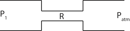
Figure 5.3.4 demonstrates a system where dissipative flow is apparent. In this case the steady-state fluid is flowing horizontally in a pipe with uniform area. Thus, there is no change in gravitational or kinetic energy-density from point 1 to point 2 in the figure. Equation \ref{dEth-IR} simplified to \(\Delta P=-IR\). The decrease in pressure from points 1 and 2 is seen here by introducing standpipes into the fluid system. A standpipe is connected to a fluid system with the top of the standpipe exposed to the atmosphere. Initially, as fluid flows past a standpipe the higher pressure of the flowing fluid will push against the air which is at a lower atmospheric pressure. The fluid will continue to rise in the standpipe until the gravitational potential energy-density difference compensates the pressure difference between between the top and the bottom of the fluid in the standpipe, and equilibrium is established.

  Figure 5.3.4: Dissipative Fluid Flow.

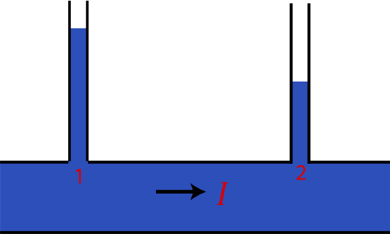
Once the system is in steady state, the fluid in a standpipe is not flowing. Although the flowing fluid system and the fluid in the standpipe indicate two different fluid systems, since one has a zero current and the other is flowing, the pressure at their boundary has to be equivalent. Thus, the height of the fluid in standpipe indirectly gives us the gauge pressure of the flowing system. For example, the difference between pressure right below standpipe marked 1 in Figure 5.3.4, \(P_1\) and atmospheric pressure is \(\Delta P=P_{atm}-P_1=\rho gh\).  The larger the height in the standpipe the greater is the pressure of the flowing fluid below, since the greater pressure is able to push more fluid upward against atmospheric pressure.  

Figure 5.3.4 shows that as the fluid flows to the right the pressure drops as seen by the drop of height of the fluid in the standpipes.  It turns out that for steady-state laminar flow resistance scales linearly with distance. Thus, the pressure drop between equidistance points would be the same as long as the properties of the pipe do not change over that segment. The longer the fluid flows the more its molecules experience frictional forces with other molecules and pipe surfaces, the greater will be the loss of its energy-density, or pressure in this case, to thermal energy.

Example \(\PageIndex{1}\)

Shown below is a segment of a pipe system in which water flows in a steady-state to the right. The wider pipes have equal areas and negligible resistance. The narrower pipe has resistance of \(2500 Js/m^6\).  For all three questions below, assume that the pressure \(P_1\) on the left is kept constant, and the pipe is open to the atmosphere on the right.   

a) You replace the narrower pipe with another pipe that has half the area and a different resistance. The water now moves 1.5 times slower in the new narrower pipe. Calculate the resistance of the new narrow pipe.

b) Now you equally increase the areas of the wider pipes (their resistance is still negligible). Everything else is as in the original set-up (not with the modified pipe from part a). Does the speed in the wider pipes increase, decrease, or stay the same? What about the speed in the narrower pipe?  

c) The original set-up is now vertical as shown below. Does the current increase, decrease, or stay the same compared to the original set-up on the top of the page?

Solution

a) The pressure difference is kept constant across this segment, so the different resistance when a new narrow pipe is placed will result in a different current.  Applying Bernoulli’s equation across the system:

\(\text{Before}: P_{\text{atm}}-P_1=-I_{\text{old}}R_{\text{old}}\)

\(\text{Before}: P_{\text{atm}}-P_1=-I_{\text{new}}R_{\text{new}}\)

Since the left-side of each equation are equal, we can set the right-side of each equation equal to each other:

\(I_{\text{old}}R_{\text{old}}=I_{\text{new}}R_{\text{new}}\)

Using \(I=Av\), we can re-write the above equation as:

\(A_{\text{old}}v_{\text{old}}R_{\text{old}}=A_{\text{new}}v_{\text{new}}R_{\text{new}}\)

and solve for \(R_{\text{new}}\):

\(R_{\text{new}}=\dfrac{A_{\text{old}}}{A_{\text{new}}}\dfrac{v_{\text{old}}}{v_{\text{new}}}R_{\text{old}}=2\times 1.5\times 2500 \dfrac{Js}{m^6}=7500 \dfrac{Js}{m^6}\)

b) If we apply Bernoulli’s equation across the system, \(P_{\text{atm}}-P_1=-IR\), increasing the area of the wider pipes does not change the current, since R is only non-zero in the narrower portion of the fluid system. Thus, the current will be the same but since \(I=Av\), the increase in area will result in a slower speed in the wider pipes. For the narrower pipe, there was no change in area, so the speed will stay the same.

c)  In this case when we apply the Bernoulli’s equation across the system:

\(P_{\text{atm}}-P_1+\rho gh=-IR\)

There is an additional gravitational potential energy-density term which is positive, when we subtract top minus bottom. Since \(\Delta P\) is kept constant, this implies that the current must decrease. Conceptually, the fluid now has to flow vertically upward, so it will flow slower (smaller flow rate), given the same pressure difference (assuming it’s sufficient to make the fluid flow uphill).

 

Adding Energy from Outside Systems: Pumps

When we are analyzing dissipative fluid-flow phenomena, we still restrict ourselves to steady-state phenomena. But without an outside source of energy, the fluid energy-density systems would gradually transfer all of their energy to the thermal energy-density system and the flow would stop. Also, how is it ever possible to make a fluid flow uphill without providing some energy source? This outside energy comes from a pump. To include pumps we add a term to the right-hand side of the extended Bernoulli equation that represents the amount of energy per unit volume transferred into the fluid energy-densities. That is, we have created an open system in which energy added from outside sources. The fully extended complete Bernoulli equation becomes:

\[ \Delta P + \rho g \Delta y + \frac{1}{2} \rho \Delta (v^2)= \dfrac{E_{\text{pump}}}{V}-IR\label{complete}\]

In biological systems an example of such as pump is the heart in our circulatory system which allows blood to flow around the body and up to the brain.

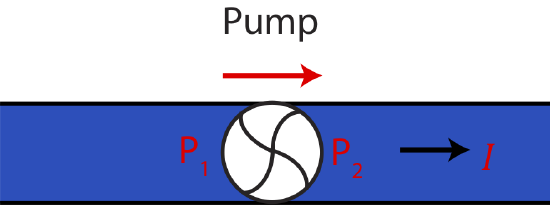
Figure 5.3.5 below shows a pump which is pumping fluid to the right (a pump must have a direction). Once the pump is turned on, and the system reaches an equilibrium steady-state, the current has to stay constant as it passes the pump. Since the pipe is horizontal and does not change area, the pump creates a greater pressure after the pump, \(P_2>P_1\), since Equation \ref{complete} simplifies to, \(\Delta P= \dfrac{E_{\text{pump}}}{V}\), assuming dissipation is negligible between points 1 and 2. Note, the term \(\dfrac{E_{\text{pump}}}{V}\) is positive as long as Bernouilli equation is analyzed in the direction of the pump.

Figure 5.3.5: Fluid Flow with a Pump.

 

Alert

We have stressed that for steady-state system the current remains constant.  However, intuitively introducing friction to your system should slow down fluid flow or introducing a pump should speed it up. How can these seemingly contradictory ideas be resolved? A constant current in steady-state systems implies that the current is the same everywhere in that particular fluid system.  But it does not imply that currents must be equal in all fluid systems. Thus, if you have a pump moving your fluid, the strength of that pump establishes the magnitude of the current which is the same before and after the pump. If you suddenly turn up the strength of the pump, you create a new fluid system with a different pump energy resulting in a faster current. This larger value of current will the same throughout this new fluid system once steady-state is reached. Likewise, if a segment of a pipe suddenly gets partially blocked, increasing the overall resistance, the fluid will slow down until it reaches a steady-state. Once the steady-state is reached and the physical properties of the system remain unchanged, the flow rate will remain the same throughout the system, even in the section with with little resistance compared to one with high resistance.

We will write the fully extended Bernoulli Equation \ref{complete} in yet one more way for several reasons. The first reason is simply to connect with experts who deal a lot with liquids, such as soil and water scientists and civil engineers, who use the term head with each of the specific terms for the fluid energy-density. These terms are pressure head, gravity head, and velocity head. Together, all three terms are called the total head. Also, rewriting Equation \ref{complete} in terms of total head, makes its similarity to electric circuits, which we discuss in the next section, more obvious. In terms of total head, the fully extended Bernoulli Equation \ref{complete} can be simply written as:

\[\Delta (\text{total head}) = \frac{E_{pump}}{V} – I R\]

We have finally arrived at the basic fluid transport equation. It can be applied along any continuous current path between whichever two points we specify. The change in the fluid energy-density (encompassed in the total head) depends explicitly, of course, on the location of the two points along the pipe. The pump term will be present if there is in fact a pump between the two chosen points. The thermal energy-density term depends on the resistance between the two points. 

Alert

Intuitively, one might think that friction slows down fluid flow and pumps speed it up. In fact, from previous analysis of conservation of energy in 7A we analyzed systems where objects slow down due to effects of friction and speed up when external forces do work on them. Therefore, when first encountering fluid dynamics it is tempting to associate effects of dissipation with a decrease in kinetic energy-density and a pump doing work on the fluid with an increase in kinetic energy-density.  However, in fluids kinetic energy-density is related with the amount fluid that flows per unit time, or the flow rate. As described in this section, the continuity equation for a steady-state system ensures that flow rate stays constant throughout the system, and kinetic energy-density can only change if the cross-sectional area of a pipe changes. This kinetic energy-density is associated with motion which is perpendicular to the cross sectional area of the pipe.  However, there is also kinetic energy-density associated with random particle motion, and we call this pressure. When a fluid enters a narrower pipe more of its motion is directed parallel to the pipe and less motion is in random directions, thus kinetic energy-density increases and pressure drops. Likewise, friction decreases the overall random motion, i.e. pressure, but the kinetic energy-density stays the same since it is fixed at a steady-state. Likewise, pumps increase pressure or the average random kinetic energy of the fluid particles, while kinetic energy-density stays the same as a consequence of conservation of mass.

 

Example \(\PageIndex{2}\)

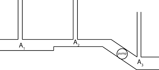
A segment of a fluid system is shown below with three equally spaced standpipes. The top of each standpipe is open to the atmosphere. The pump is pumping water downhill. The areas in regions 1 and 3 are equal, and the area in region 2 is smaller: \(A_2<A_1=A_3\). Region 3 is lower in height than regions 1 and 2.

a) Assuming there is no resistance in the pipe, rank the water levels in each stand pipe.

b) The pipe system becomes eroded, so resistance becomes significant and is uniform throughout the pipe. Assume speed of the fluid in region 1 is \(0.5 m/s\), \(A_1=4cm^2\), and \(A_2=2cm^2\). The water level decrease from standpipe 1 to 2 by \(0.3m\), and then increase from standpipe 2 to 3 by \(1.2m\). The height difference between regions 2 and 3 is \(70cm\).  Assume water is flowing through the pipe with density, \(\rho_{water}\sim 1000 kg/m^3\). Find the resistance of the horizontal pipe between regions 1 and 3, and find the energy of the pump per unit volume. Show your work.

 

Solution

a) Writing down only the non-zero terms of the full Bernoulli's equation between regions 1 and 2:

\(\Delta P+\Delta KE=0\)

Since the area decreases from 1 to 2, the speed will increase, \(A_1v_1=A_2v_2\), resulting in an increase of kinetic energy-density. Therefore, the pressure must decrease, \(P_2<P_1\).

Between regions 2 and 3, the Bernoulli's equation is:

\(\Delta P+\Delta KE+\Delta PE_g=\dfrac{E_{pump}}{V}\)

Since the area increases from 2 to 3, the speed will decrease resulting in a decrease of kinetic energy-density. The height is lower in region 3, so the gravitational potential energy will also decrease. The pump adds energy to the system, thus, the left side of the equation must be positive. Since the other two terms are both negative, the change in pressure must be positive. Therefore, the pressure must increase, \(P_3>P_2\).

Between regions 1 and 3, the Bernoulli's equation is:

\(\Delta P+\Delta PE_g=\dfrac{E_{pump}}{V}\)

The argument is the similar to above, except there is no change in area. Thus, since the change in gravitational potential energy-density is negative, and the pump adds energy to the system, the pressure must increase, \(P_3>P_1\).

Putting the three results together we find, \(P_3>P_1>P_2\). The higher the pressure, the higher will be the height in each standpipe, so \(h_3>h_1>h_2\).

b) Use the given information for region 1 to find the flow rate:

\(I=A_1v_1=4\times 10^{-4}m^2\times0.5 m/s =2\times 10^{-4} m^3/s\).

The speed in region 2 can be found using the continuity equation, \(A_1v_1=A_2v_2\):

\(v_2=v_1\dfrac{A_1}{A_2}=0.5 m/s\times 2= 1.0 m/s\).

The pressure difference between the standpipes can be determined from the height difference information. Below each standpipe the pressure is, \(P_{below}=P_{atm}+\rho g h\), where h is the height of the fluid level in the stand pipe. The difference between any two standipes is related to the difference in the heights of the fluids that fill the standpipes, \(\Delta P=\rho g \Delta h\).

There are two unknowns here, the resistance and the pump energy. Thus, first solve for the resistance between regions 1 and 2, since there is no pump present in this region:

\(\Delta P+\Delta KE=-IR\)

\(R_{12}=-\dfrac{\Delta P_{12}+\Delta KE_{12}}{I}=-\dfrac{\rho g(h_2-h_1)+\frac{1}{2}\rho (v_2^2-v_1^2)}{I}=-\dfrac{1000 kg/m^3\times 10 m/s^2\times(-0.3m)+\frac{1}{2}\times 1000 kg/m^3 \times(1.0^2-0.5^2)m^2/s^2}{2\times 10^{-4} m^3/s}= 1.3 \times 10^7 \dfrac{Js}{m^6}\).

Since the standpipes are equally spaces and resistance is uniform, the total resistance between standpipes 1 and 3 is double the resistance between regions 1 and 2. So, \(R_{13} = 2.6 \times 10^7 Js/m^6\). Applying Bernoulli's equation between regions 1 and 3 to find the pump energy-density:

\(\Delta P_{13}+\Delta PE_{g,13}=\dfrac{E_{pump}}{V}-IR_{13}\)

\(\dfrac{E_{pump}}{V}=\rho g(h_3-h_1)+\rho g(y_3-y_1)+IR_{13}=1000 kg/m^3\times 10 m/s^2\times 0.9m+1000 kg/m^3\times 10 m/s^2\times (-0.7m)+2\times 10^{-4} m^3/s\times 2.6 \times 10^7 Js/m^6=7200 \dfrac{J}{m^3}\)

In the equation above \(\Delta h=h_3-h_1\) is the height difference between the water levels in standpipes 3 and 1. Since the water levels drops from 1 to 2 by 0.3m and then increases from standpipe 2 to 3 by 1.2m, \(h_3-h_1=0.9m\). The height difference between regions 2 and 3 is \(\Delta y=y_3-y_1=-70cm=-0.7m\).

 

Power in Relation to Fluid Flow

In general, power is simply the rate of energy transfer. Each term in our fluid transport equation represents either a change in an energy-density \(\Delta P\), \(\Delta PE_g/V\), and \(\Delta KE/V\)) or a transfer of energy per unit volume of fluid \(IR\) and \(E_{\text{pump}}/V \)). If we want to determine the amount of energy change that occurs in the fluid as it passes between two points along a pipe per time, we need to multiply the energy change per volume by the volume of fluid passing through the pipe and divide by the time. But volume divided by time is just the current. So the power associated with each energy-density term, is simply the the change in energy-density multiplied by the current. In the case of transfer terms, power is simply the energy transferred per volume multiplied by the current:

\[ Power =\dfrac{\Delta E}{t}=\dfrac{\Delta E}{V}\times\dfrac{V}{t}=\dfrac{\Delta E}{V}I\]

It is almost universal to use the symbol \(P\) for power, and we will follow this custom. You will need to be sensitive to the context of the equation to know whether \(“P”\) means power or pressure. This will not be confusing, if you always think about the meaning of the equation in which \(“P”\) appears.

Exactly how we algebraically express power will depend, of course, on the particular context, i.e., exactly which section of the pipe or channel we are focusing on and which energy-density system we are focusing on. There is not one single expression. Rather, we have to use the basic meaning of power and apply it appropriately to each context. Several of these are listed below.

Rate of change of all fluid energy densities:

\[P = |\Delta (\text{total head})| I\]

Rate at which energy is transferred into the fluid by a pump:

\[P = \dfrac{E_{pump}}{V}  I \]

Rate energy is transferred into the thermal energy-density from the fluid energy densities:

\[P =I^2R \]

Contributors

• Authors of Phys7A (UC Davis Physics Department)