
7.3: Angular Motion
- Page ID
- 51946

\( \newcommand{\vecs}[1]{\overset { \scriptstyle \rightharpoonup} {\mathbf{#1}} } \)
\( \newcommand{\vecd}[1]{\overset{-\!-\!\rightharpoonup}{\vphantom{a}\smash {#1}}} \)
\( \newcommand{\id}{\mathrm{id}}\) \( \newcommand{\Span}{\mathrm{span}}\)
( \newcommand{\kernel}{\mathrm{null}\,}\) \( \newcommand{\range}{\mathrm{range}\,}\)
\( \newcommand{\RealPart}{\mathrm{Re}}\) \( \newcommand{\ImaginaryPart}{\mathrm{Im}}\)
\( \newcommand{\Argument}{\mathrm{Arg}}\) \( \newcommand{\norm}[1]{\| #1 \|}\)
\( \newcommand{\inner}[2]{\langle #1, #2 \rangle}\)
\( \newcommand{\Span}{\mathrm{span}}\)
\( \newcommand{\id}{\mathrm{id}}\)
\( \newcommand{\Span}{\mathrm{span}}\)
\( \newcommand{\kernel}{\mathrm{null}\,}\)
\( \newcommand{\range}{\mathrm{range}\,}\)
\( \newcommand{\RealPart}{\mathrm{Re}}\)
\( \newcommand{\ImaginaryPart}{\mathrm{Im}}\)
\( \newcommand{\Argument}{\mathrm{Arg}}\)
\( \newcommand{\norm}[1]{\| #1 \|}\)
\( \newcommand{\inner}[2]{\langle #1, #2 \rangle}\)
\( \newcommand{\Span}{\mathrm{span}}\) \( \newcommand{\AA}{\unicode[.8,0]{x212B}}\)
\( \newcommand{\vectorA}[1]{\vec{#1}} % arrow\)
\( \newcommand{\vectorAt}[1]{\vec{\text{#1}}} % arrow\)
\( \newcommand{\vectorB}[1]{\overset { \scriptstyle \rightharpoonup} {\mathbf{#1}} } \)
\( \newcommand{\vectorC}[1]{\textbf{#1}} \)
\( \newcommand{\vectorD}[1]{\overrightarrow{#1}} \)
\( \newcommand{\vectorDt}[1]{\overrightarrow{\text{#1}}} \)
\( \newcommand{\vectE}[1]{\overset{-\!-\!\rightharpoonup}{\vphantom{a}\smash{\mathbf {#1}}}} \)
\( \newcommand{\vecs}[1]{\overset { \scriptstyle \rightharpoonup} {\mathbf{#1}} } \)
\( \newcommand{\vecd}[1]{\overset{-\!-\!\rightharpoonup}{\vphantom{a}\smash {#1}}} \)
\(\newcommand{\avec}{\mathbf a}\) \(\newcommand{\bvec}{\mathbf b}\) \(\newcommand{\cvec}{\mathbf c}\) \(\newcommand{\dvec}{\mathbf d}\) \(\newcommand{\dtil}{\widetilde{\mathbf d}}\) \(\newcommand{\evec}{\mathbf e}\) \(\newcommand{\fvec}{\mathbf f}\) \(\newcommand{\nvec}{\mathbf n}\) \(\newcommand{\pvec}{\mathbf p}\) \(\newcommand{\qvec}{\mathbf q}\) \(\newcommand{\svec}{\mathbf s}\) \(\newcommand{\tvec}{\mathbf t}\) \(\newcommand{\uvec}{\mathbf u}\) \(\newcommand{\vvec}{\mathbf v}\) \(\newcommand{\wvec}{\mathbf w}\) \(\newcommand{\xvec}{\mathbf x}\) \(\newcommand{\yvec}{\mathbf y}\) \(\newcommand{\zvec}{\mathbf z}\) \(\newcommand{\rvec}{\mathbf r}\) \(\newcommand{\mvec}{\mathbf m}\) \(\newcommand{\zerovec}{\mathbf 0}\) \(\newcommand{\onevec}{\mathbf 1}\) \(\newcommand{\real}{\mathbb R}\) \(\newcommand{\twovec}[2]{\left[\begin{array}{r}#1 \\ #2 \end{array}\right]}\) \(\newcommand{\ctwovec}[2]{\left[\begin{array}{c}#1 \\ #2 \end{array}\right]}\) \(\newcommand{\threevec}[3]{\left[\begin{array}{r}#1 \\ #2 \\ #3 \end{array}\right]}\) \(\newcommand{\cthreevec}[3]{\left[\begin{array}{c}#1 \\ #2 \\ #3 \end{array}\right]}\) \(\newcommand{\fourvec}[4]{\left[\begin{array}{r}#1 \\ #2 \\ #3 \\ #4 \end{array}\right]}\) \(\newcommand{\cfourvec}[4]{\left[\begin{array}{c}#1 \\ #2 \\ #3 \\ #4 \end{array}\right]}\) \(\newcommand{\fivevec}[5]{\left[\begin{array}{r}#1 \\ #2 \\ #3 \\ #4 \\ #5 \\ \end{array}\right]}\) \(\newcommand{\cfivevec}[5]{\left[\begin{array}{c}#1 \\ #2 \\ #3 \\ #4 \\ #5 \\ \end{array}\right]}\) \(\newcommand{\mattwo}[4]{\left[\begin{array}{rr}#1 \amp #2 \\ #3 \amp #4 \\ \end{array}\right]}\) \(\newcommand{\laspan}[1]{\text{Span}\{#1\}}\) \(\newcommand{\bcal}{\cal B}\) \(\newcommand{\ccal}{\cal C}\) \(\newcommand{\scal}{\cal S}\) \(\newcommand{\wcal}{\cal W}\) \(\newcommand{\ecal}{\cal E}\) \(\newcommand{\coords}[2]{\left\{#1\right\}_{#2}}\) \(\newcommand{\gray}[1]{\color{gray}{#1}}\) \(\newcommand{\lgray}[1]{\color{lightgray}{#1}}\) \(\newcommand{\rank}{\operatorname{rank}}\) \(\newcommand{\row}{\text{Row}}\) \(\newcommand{\col}{\text{Col}}\) \(\renewcommand{\row}{\text{Row}}\) \(\newcommand{\nul}{\text{Nul}}\) \(\newcommand{\var}{\text{Var}}\) \(\newcommand{\corr}{\text{corr}}\) \(\newcommand{\len}[1]{\left|#1\right|}\) \(\newcommand{\bbar}{\overline{\bvec}}\) \(\newcommand{\bhat}{\widehat{\bvec}}\) \(\newcommand{\bperp}{\bvec^\perp}\) \(\newcommand{\xhat}{\widehat{\xvec}}\) \(\newcommand{\vhat}{\widehat{\vvec}}\) \(\newcommand{\uhat}{\widehat{\uvec}}\) \(\newcommand{\what}{\widehat{\wvec}}\) \(\newcommand{\Sighat}{\widehat{\Sigma}}\) \(\newcommand{\lt}{<}\) \(\newcommand{\gt}{>}\) \(\newcommand{\amp}{&}\) \(\definecolor{fillinmathshade}{gray}{0.9}\)Overview
In the next few sections we will see that the ideas we have developed for linear momentum and impulse apply to rotational motion as well. To describe rotational or angular motion we will need to develop rotational analogs of the various variables and concepts we have been using. Force, acceleration, momentum, velocity, and impulse all have rotational analogs. Newton's Laws, the concept that impulse equals change in linear momentum, the principle of conservation of momentum all have analogs in rotational motion.
In the impulse-momentum model, we focused both on the properties of forces and the momentum transfers governing the connection of force to motion. Now we extend the formalism to enable us to analyze and make sense of the motion of extended objects that can rotate as well as translate. When objects translate, we say that they have linear momentum. When objects rotate, we will describe their motion with angular momentum (which could also be called "rotational momentum"). We will introduce a couple of additional concepts: torque (rotational analog of force) and rotational inertia (rotational analog of mass).
Although torque arises directly from the presence of a force, it is a rather different quantity. We will see that not all forces result in torques, and that torque also depends on the exact location of where the force is applied. Even the units of torque are different from the units of force. Angular momentum is analogous to momentum (translational or linear momentum) but the two types of momentum describe different physical situations. The impulse-momentum model stated that the momentum of an object is conserved if there is no net external force acting on it. We will find that angular momentum of an object is conserved if there is no net external torque acting on it (even if there is a net force). Similarly, a transfer of angular momentum is called angular impulse.
Translational or linear and angular motion describe different physical situations, although there is a connection between them. The difference is obvious when you see a physical situation but, when discussing abstract ideas without a physical picture in mind, it is easy to confuse the two quantities. For instance, a ball may be spinning (i.e. have angular momentum) and flying through the air in a straight line (i.e. have linear momentum). Or it may be spinning (have any angular momentum) and not be flying through the air. Or it may be flying through the air but not spinning at all. So, you see that the amount of angular momentum the ball has is completely independent of its linear momentum. The moral of this little story is the same as with all physics problems: try to keep a concrete physical picture in your head as you learn new abstract ideas.
Rotational Velocity
We begin by developing some useful relationships to describe the motion of a point object. Figure 7.3.1 shows a wheel, with radius \(R\) which rotates around its center. The question that we want to ask is how do we describe the motion of the wheel. We can attempt to use our developed ideas of linear velocity. Let us focus on two arbitrary points on the wheel (marked with red and blue points in the figure). The direction of the velocity of each point is tangent to the circle since the wheel rotates about its center. The magnitude of the two velocities will be different. The red dot on the outer rim moves the entire circumference of the wheel, \(2\pi r\), over the same period of time as the blue dot moves a much smaller distance, since it covers a smaller circumference being closer to the center of the wheel.
Figure 7.3.1: Rotational Analog of Velocity
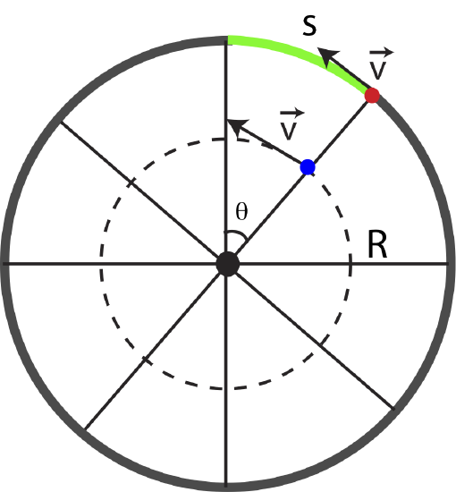
Thus, if we use these two different points to describe the motion of the wheel, we would obtain different answer. And even more extreme, if we choose to focus on the center of the wheel, it does not move at all, so we conclude the velocity is zero. This is exactly what leads us to the distinction between angular and linear motion. When we discussed linear motion, we always stated that we can "collapse" an extended object to a point and only think about the motion of the point. Likewise, all the forces acting on the object were treated as if they were all applied at one location, the point representing the extended object. If we redefine this wheel as just a point object at the center, we conclude that it has zero linear motion. This makes sense since the wheel is not translating in space, its center remains in the same location as it rotates. In fact, we can attempt to add up all the velocities of all the points on the wheel, and we would find that they all cancel. For example, there is an analog of a red dot on the opposition side of the wheel that moves in the opposite direction with the same speed, so the sum of those two velocities is zero. Equivalently, the same analog exists for the blue dot and all other points on the wheel.
So we have concluded that the wheel's linear velocity, \(\vec v\), is zero. But the wheel is clearly not stationary, it is rotating, so there must be more information that we can provide to describe the motion. Let us think about what is the same for the red and the blue dots. Even though their velocities are different, they cover the same angle, \(\theta\), during the same amount of time. Thus, instead of describing a linear displacement, \(\Delta x\), per unit time, we will use an an angular displacement, \(\Delta\theta\), per using time. In Figure 7.3.1 the angle is measured relative to some arbitrarily chosen axis which is frequently measured from the positive x axis, but it could be measured from any reference line. Recall, we define linear speed as the rate of change of a small displacement over time. Analogously, we define angular speed, \(\omega\), as the rate of change of a small change in angle over time:
\[v=\dfrac{dx}{dt}~\Longleftrightarrow~\omega=\frac{d\theta}{dt}\label{omega}\]
When the wheel in Figure 7.3.1 rotates by some angle \(\theta\), the red point move by a distance of arc length, \(s\), as illustrated by a green color in the figure. Since the change in angle is describing the same motion as the change in distance, we can connect the two using a known geometric relationship between angle, \(\theta\), radius, \(R\), and arc length, \(s\):
\[s=R\theta\label{arc}\]
Combining Equations \ref{omega} and \ref{arc}, and substituting displacement \(dx\) with change in arc length, \(ds\), we obtain a relationship between angular and linear speed:
\[v=\frac{ds}{dt}=R\frac{d\theta}{dt}=R\omega\]
The result above is consistent with our original discussion, the red dot on the outer rim of the wheel has a larger speed since further from the center compared to the green dot. Both points has the same angular speed, so the red dot with have a greater linear speed since the distance \(R\) is greater for the red dot.
The units of \(\theta\) and \(\omega\) are, respectively, an angle unit and an angle unit divided by time. We can use any units we want and that are useful for a particular application of rotational motion. Typical units for angular speed are degrees/second, revolutions/second, revolutions/hour, etc. The SI units, are, however, radians for angle and radians per second for angular speed. We must use radians and radians per second when we use the relationship connecting \(v\) to \( \omega \). Note that a “radian” is a rather unique kind of unit. For instance, radians multiplied by meters is just meters, not rad·meters. A wheel which makes 5 revolutions per second, in radians will move at an angular speed of \(10\pi~\textrm{rad/sec}\), since each full revolution is \(2\pi\) in radians.
Note that so far we have been discussing objects constrained to move in a circle. We defined that motion in terms of polar coordinates, using the radial distance from the origin, \(r\), and the angle relative to the positive x-axis, \(\theta\). We can also describe the kinematics of any extended object (e.g. a baseball bat) that is rotating about a fixed origin (where we grip it) by \(\theta\) and \(\omega\) , as long as we define the coordinates about the fixed axis of rotation.
Extending the connection of linear and angular speed to acceleration, we can define an angular acceleration, \(\alpha\), which describes the rate of change of angular velocity:
\[\alpha=\frac{d\omega}{dt}\]
Similarly, we can connect linear and angular accelerations:
\[a=\frac{dv}{dt}=R\frac{d\omega}{dt}=R\alpha\]
When forces act on extended objects, in addition to causing changes in translational motion, but can also cause changes in rotational motion. That is, these forces can cause translational acceleration and/or angular acceleration. It turns out that it is not just the magnitude and direction of the force that is important in causing angular accelerations, but also where the force is applied on an extended object. Torque is the angular analog of force that incorporates both the force vector as well as where it is applied to an object. We will define torque in greater detail in the coming sections.
So far we have conveniently ignored the direction aspect of angular velocity and purely focused on speed. Just as the translational velocity vector, \(\vec v\), describes both direction and magnitude, the angular velocity, \(\vec\omega\), is also a vector. What direction does angular velocity have? Looking back at the wheel in Figure 7.3.1, we can summarize its motion as counter-clockwise. But this description or rotation (clockwise or counter-clockwise) is not a direction in a particular spatial coordinate. In addition, there is another problem. If another observer is standing on the other side of the wheel, then they would describe the motion as clockwise, and there there would be a disagreement. And how would you distinguish its rotational direction is the wheel was horizontally positioned instead? The only unique direction in space associated with a rotation is along the axis of rotation, which is an axis perpendicular to the plane of rotation. For the wheel in Figure 7.3.1 the axis of rotation would be a line which is perpendicular to the screen, going in and out of the screen.
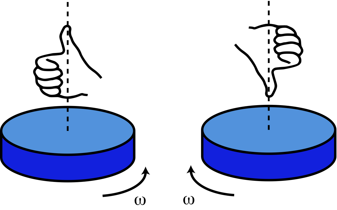
So, if the axis of rotation gives the direction, the only thing left to specify which way along the axis corresponds to a particular direction of rotation. For the wheel in Figure 7.3.1, we want to know whether the counter-clockwise rotation corresponds to a direction which is in or out of the page. By convention, the direction is specified by the right-hand-rule (RHR). If you curl the fingers of your right hand in the direction of positive \(\theta\) or in the direction rotation is occurring, your thumb points in the direction (along the axis of rotation) of \(\theta\) or \(\omega\). For the wheel in Figure 7.3.1 the RHR (fingers curl to the left so thumb stick out of the page) would result in angular velocity pointing out of the page. Figure 7.3.2 below shows several examples of the right-hand-rule. On the left, a cylinder is rotation counter-clockwise as viewed from above. A right hard is shown with the fingers curled in the direction of rotation, resulting in the thumb pointing up. So, we conclude that the direction of rotation is in the positive vertical direction. On the contrary, the cylinder on the right is rotating clockwise as seen from above. In this case the RHR gives us the direction of angular velocity to be in the negative vertical direction.
Figure 7.3.2: Right Hand Rule for Rotational Motion
Alert
The direction of angular velocity does not specify the direction in which the object is physically rotating. In fact, it is always the direction in which no motion is occurring since it is the only unique direction for the entire span of rotation.