10.7: Multiple Optical Devices

Often to utilize the power of optical devices, multiple devices are used in combination to create images. The figure below shows an example of an object placed in front of two lenses, the first converging lens with focal point \(f_1\) followed by a diverging lens with focal point \(f_2\) placed a distance, \(d\), apart. Our goal is to use tools of ray tracing, the thin-lens/mirror equation, and the magnification equation we applied to single optical device to determine image positions, types, and magnification of a multiple device system.

Figure 10.7.1: Two Lens System

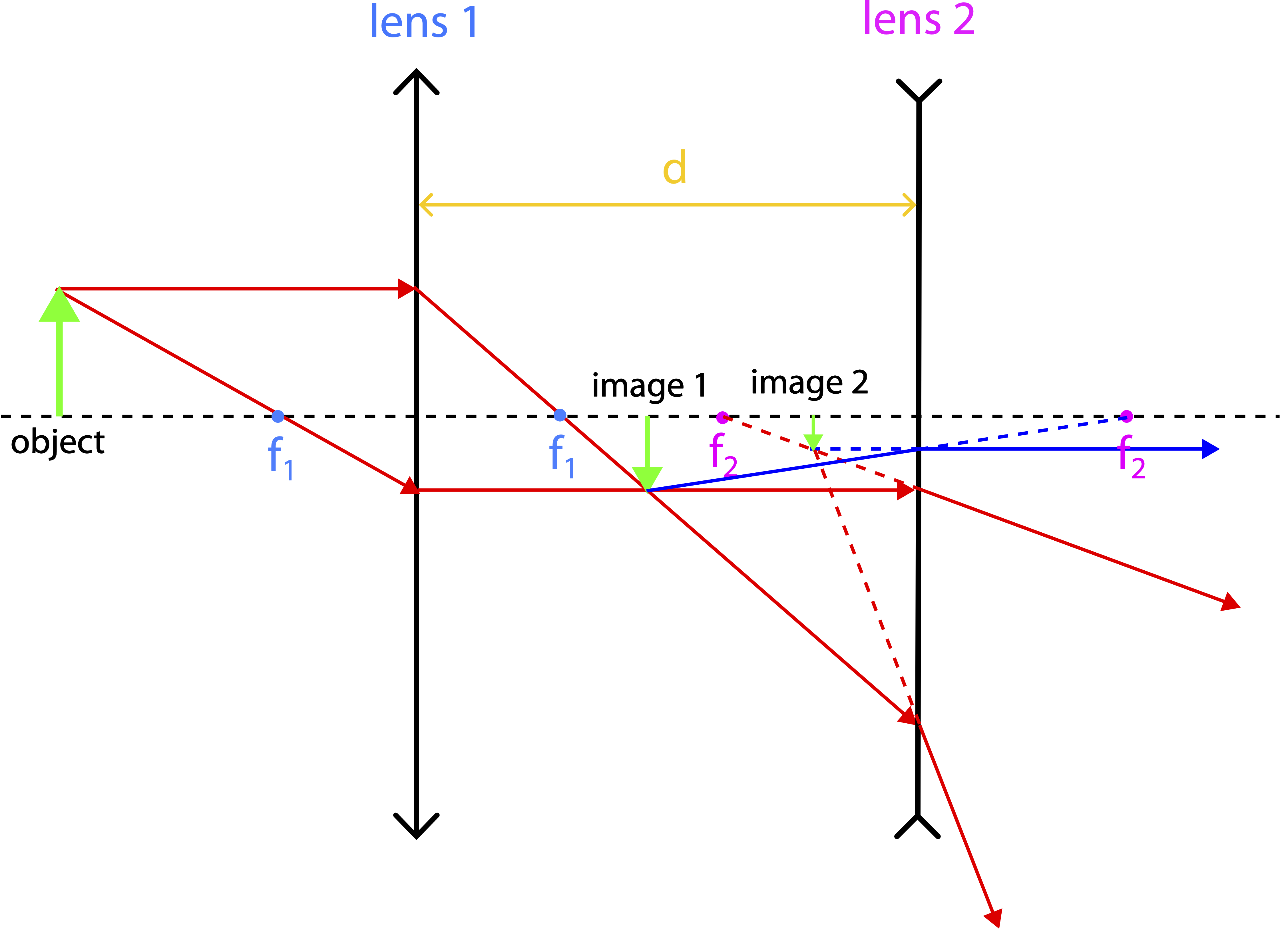
In the figure light from the object will go through the first lens a governed by the single-lens ray tracing. In order to not overcrowd the image, only two of the three principle rays are shown above. The first lens is a converging lens, and since the object is placed further than the focal point, the image formed will be real, inverted, and on the opposite side of the the lens. This image is labeled "image 1" in the figure.

The rays that create the first image continue traveling and refract through the second lens. When red principle ray that refracts parallel to the optical axis encounters lens two, it is one of the principle rays for this lens as well, so we can readily determine how it will refract. Since lens 2 is a diverging lens, it will refract away from the near focal point. The other red principle ray from lens 1 is not one of the three principle rays for lens 2, so it is not easy to determine how it will refract.

However, there are many rays that pass through the first image and encounter the second lens. Some of these rays will be the principle rays for the second lens. Thus, we can draw the principle rays coming from image 1 to determine how lens 2 will form the final image. The blue ray is the second principle ray for lens 2, traveling toward the far focal point of lens 2, and refracting parallel to the optical axis. In other words, the first image become the object for the second lens.  From these rays we can see that they will not converge behind lens 2, but can be traced back in front of lens 2 to create image 2.

The final image is an inverted virtual image. Although, one lens cannot make an inverted image which is virtual, this can occur with a multiple lens system. The first image was real and inverted, and the following virtual image keeps the orientation of the first image, so it remains inverted. For completeness, we show in the figure the other red ray that was not a principle ray for lens 2, refracting through lens 2. Since all rays participate in creating the image, the refracted ray will bend in such as way that it traces back to image 2, as shown.

Mathematically, we can treat this system as two independent single-lens systems. Initially, when the first lens makes the image, the location of that image can be calculated as follows:

\[\dfrac{1}{f_1}=\dfrac{1}{o_1}+\dfrac{1}{i_1}\]

where \(o_1\) is the distance from the object to lens 1, \(f_1\) is the focal length of lens 1, and \(i_1\) is the distance of the image to lens 1. Next, we treat image 1 as the object for lens 2:

\[\dfrac{1}{f_2}=\dfrac{1}{o_2}+\dfrac{1}{i_2}\]

One thing that one must be careful about is connecting the image from lens 1 to the objects for lens 2. The image distance \(i_1\) is the distance of the image from lens 1, while the object distance \(o_2\) must be the distance of the object from lens 2.  But the two quantities can be related when the distance \(d\) between the two lenses is known:

\[o_2=d-i_1\label{o2}\]

When \(i_2\) is positive as in the case in Figure 10.7.1, then the object distance for lens 2 is simply the difference between the distance between the lenses and the distance of image 1 to lens 1. If the first lens made a virtual image on the same side as the original object of the lens, then the object distance to lens 2 would become the distance between the two lenses plus the distance of the first image to lens 1. Equation \ref{o2} would still apply since \(i_1<0\) for virtual images, so the subtraction becomes an addition as expected.

For total magnification we want to compare the size of the final image to the size of original object:

\[M_{\text{tot}}=\dfrac{h_{i_2}}{h_{o_1}}\label{Mtot}\]

We would also like to determine how the total magnification relates to the object and image distances. To do this we first look at the magnification, \(M_1\) by lens 1:

\[M_1=\dfrac{h_{i_1}}{h_{o_1}}=-\dfrac{i_1}{o_1} \rightarrow h_{i_1}=-\dfrac{i_1}{o_1}h_{o_1}\]

Similarly the second magnification, \(M_2\):

\[M_2=\dfrac{h_{i_2}}{h_{o_2}}=-\dfrac{i_2}{o_2} \rightarrow h_{i_2}=-\dfrac{i_2}{o_2}h_{o_2}\]

The height of the first image become the height of the second object, \(h_{i_1}=h_{o_2}\). Combing the two equations above we find:

\[h_{i_2}=\left(-\dfrac{i_2}{o_2}\right)\left(-\dfrac{i_1}{o_1}\right)h_{o_1}\]

And plugging back into Equation \ref{Mtot} for the total magnification we find:

\[M_{\text{tot}}=\left(-\dfrac{i_1}{o_1}\right)\left(-\dfrac{i_2}{o_2}\right)=M_1\cdot M_2\]

More generally, for a system of N-lenses the total magnification equation is:

\[M_{\text{tot}}=M_1\cdot M_2\cdot...\cdot M_N=\prod_{n=1}^{N}M_n\]

If there are more than two optical devices, you follow the same procedure as you would for the two devices. The second image becomes the object for the third device, and so on. There are situations where an image by the first lens is made on the other side of the second lens. This is a situation of a virtual object which we will not cover in this course. Thus, we will only look at scenarios where the first image is created in front of the second lens.

Example \(\PageIndex{1}\)

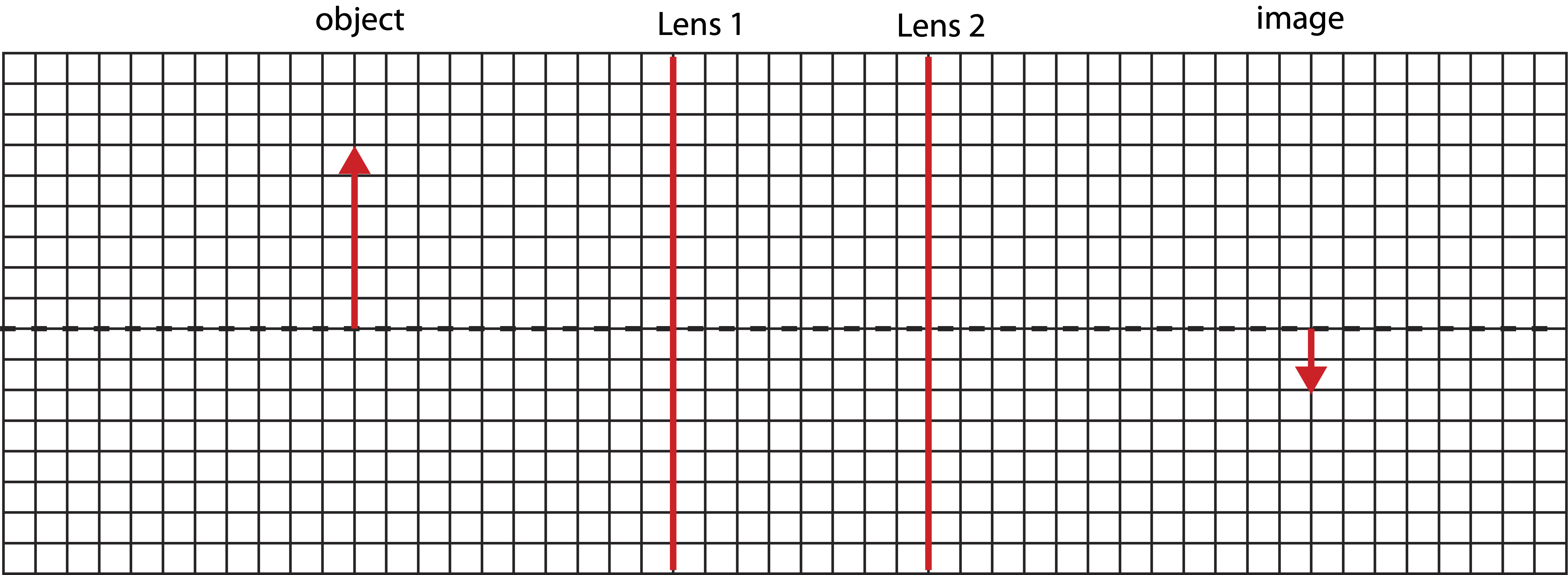
Bellow is a set up with two lenses of unknown types and focal lengths. The object and final image are shown. The heights of the object and image and all the distances are drawn to scale (each grid represents 1 cm in distance). Determine the type and the focal length of each lens.

Solution

The final image is real since it is on the other side of lens 2. Thus, lens 2 is converging. Since it's inverted from the original object, the first image had to be upright. Thus, the first image is virtual, which means that lens 1 can be either diverging or converging. So we need to do further calculations to determine the nature what type is lens 1.

Let's first gather what information is given in the figure. The object is 10 cm away from lens 1: \(o_1=10 cm\). The two lenses are 8 cm apart: \(d=8 cm\). The final image is 12 cm to the right of lens 2: \(i_2=12 cm\). Also, the height of the object is 6m, and the height of the final image is -2 cm. From the heights we can determine the total magnification is:

\[M_{tot}=\dfrac{h_{i_2}}{h_{o_1}}=-\dfrac{2}{6}=-\dfrac{1}{3}=\left(-\dfrac{i_1}{o_1}\right)\left(-\dfrac{i_2}{o_2}\right)=\left(\dfrac{i_1}{10 cm}\right)\left(\dfrac{12 cm}{8 cm -i_1}\right)=\dfrac{6}{5}\cdot\dfrac{i_1}{8-i_1}\nonumber\]

From the above equation we can solve for \(i_1\):

\[5(i_1-8)=18i_1 \rightarrow i_1=-\dfrac{40}{13} cm \nonumber\]

Since we know the object distance for lens 1, we can now solve for the focal point of lens 1:

\[\dfrac{1}{f_1}=\dfrac{1}{o_1}+\dfrac{1}{i_1}=\dfrac{1}{10}-\dfrac{13}{40} \rightarrow f_1=-\dfrac{9}{40} cm \nonumber\]

Thus, lens 1 is diverging since the focal length is negative. Since we know the location of image 1, we can find the location of object 2:

\[o_2=8cm+\dfrac{40}{13}cm=\dfrac{144}{13}cm \nonumber\]

Finally, solving for the focal length of lens 2:

\[\dfrac{1}{f_2}=\dfrac{1}{o_2}+\dfrac{1}{i_2}=\dfrac{13}{144}+\dfrac{1}{12} \rightarrow f_2=5.76 cm \nonumber\]