8.3: Multi-Dimensional Waves

Sound Waves

Sound is a wave in the sense that we have already defined. However, sound waves in air behave differently from the material waves we have described so far. As we discussed in Physics 7A the bonds between particles in the air are virtually non-existent, so the particles in the medium are non-interacting and do not exert forces on each other. The oscillations in the medium can no longer be described in terms of restoring forces modeled by Hooke's Law. Instead, we can explain how sound wave propagate through air in terms of variations in pressure. In other words, a sound wave can be described as a pressure wave. The pressure variations occur in the same direction as wave propagation, so sound waves are longitudinal. 

Although, individual air particles do not oscillate about some equilibrium position, as a sound wave travels through air the oscillation occur in the density or the pressure of the air. We learned in Physics 7A that air molecules move around rapidly in random motion, but there are well-defined averages for density and pressure. Sound waves in air are the oscillation of the average value of particle density (and therefore pressure) over distance scales much larger than the mean distance between particles. Thus we can model sound wave considering only the pressure or density of the air.

While this is slightly different in form from the material waves, we can apply almost all of the same techniques that we have already learned to sound waves. Fundamentally, however, sound waves are just material waves in a medium and so we may not be surprised that the same techniques work.

Choosing pressure to describe sound waves, the sound wave equation becomes:

\[P(x,t) -P_{atm}= P_o \sin{\left(\dfrac{2\pi }{T}t \pm \dfrac{2\pi}{\lambda}x + \phi_o \right)}\]

where \(P(x, t)\) is the absolute pressure of the air at a given position \(x\) and at a time \(t\). \(P_{atm}\) is the atmospheric pressure (i.e. the equilibrium pressure). \(P_o\) is the amplitude of the pressure fluctuation (gauge pressure) from equilibrium, such that when the displacement is at a crest, the pressure is at a maximum of \(P_{atm}+P_o\), and when it's at a trough, the pressure is at a minimum of \(P_{atm}-P_o\).

Note the similarities between this equation in terms of pressure and Equation \ref{wave-equation} in terms of individual particle displacement. We can therefore ascribe familiar parameters to sound waves, such as wavelength, period, and wave speed. We can also use the same techniques from the previous section to plot the pressure against time at constant position, or pressure against position at constant time.

Wavefronts and Rays

The wave equation we introduced in the previous section describes one-dimensional waves. However, in most cases waves propagate in either two-dimensions (such as the surface of water) or in three-dimensions (such as sound or light). Although, we will not introduce the mathematical representation of higher dimensional waves in this course, there are other representations for multi-dimension waves which are useful. The figure belows shows a drawing of two-dimensional wavefronts, concentric circles are crests (solid lines) and troughs (dashed lines) emanating from the source located at the center. The wavefornts spread as they move away from the source, like ripples in a pond.

Figure 8.3.1: Wavefronts and Rays

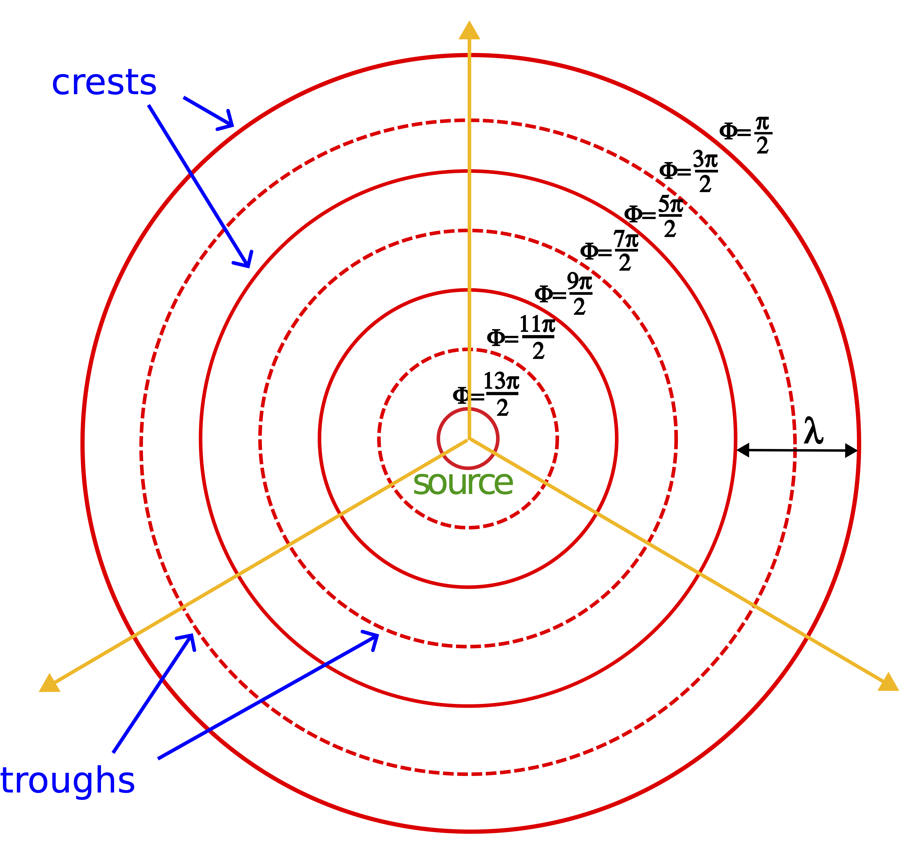
This is a snapshot representation of the location of crests and troughs at a specific time. At a later time, each wavefront would be found further from the source and more wavefronts would be shown as new crests are troughs are generated by the source. Each wavefront provides information about the relative times that they were generated Since the wavefronts move outward, the wavefront which is furthest from the source was the first one that was generated, and the one closest to the source is the last one to be emitted. Thus, time "increases inward" from the furthest to the closest wavefront. If we define \(x=0\) m to be the location of the source, and \(t=0\) s is the time the first crest was generated, then the total phase of the furthest crest is \(\pi/2\). The furthest trough was generated half a cycle later, at \(t=T/2\) s, so the total phase is bigger than that of the first crest's by \(\pi\), resulting in a total phase of \(3\pi/2\). The phase of the next crest is a full cycle larger, or \(2\pi\) bigger than the phase of the first crest, and so on. The wavefront representation stresses that the total phase is a characteristic of a specific part of the wave.

The wavefront representation also contains information about the spacial periodicity of the wave, since distance between any neighboring crests or troughs is one wavelength. However, since this is a snapshot, information about the temporal periodicity, period or frequency, is lost in this representation. Also, since this is a "top view" of the wave propagating in two-dimensions, information about amplitude cannot be obtain from this picture. In fact, as we will see shortly, amplitude is no longer a constant in higher dimensional waves. Although complete information about the wave in lost in this representation, it is often an informative tool for understanding certain wave phenomena, such as interference introduced in later sections. In three-dimensions the concentric circles in Figure 8.3.1 would become concentric spherical shells. 

The arrows drawn in the figure provide yet another useful wave representation. The arrows only preserve the information about wave direction. They are always drawn perpendicular to the wavefronts and point in the direction of wave motion. This representation will be especially useful when we discuss optics as an application of various properties of light. Various optical phenomena that we will study mostly arise due to the direction of the motion of rays of light. Thus, the most useful representation for that unit will be the ray representation.

Most waves in nature are multi-dimensional. The only truly one-dimensional wave are those confined to a string or rope. However, the one-dimensional wave representation is often a good approximation to multi-dimensional waves far away from the source. Imagine an observer standing far away from a wave source and can only detect a small area of the wavefronts. This is represented by the dashed rectangle in the figure below. To this observer the individual wavefronts look almost parallel. The further the observer is from the source, the smaller portion of the wavefronts they can detect, the more parallel the wavefronts will appear. If the wavefronts are parallel that means the wave is moving in one direction perpendicular to the wavefronts. This is illustrated on the right "zoomed-in" picture of the wavefronts far from the source. The rays which are perpendicular to the wavefronts are all parallel, implying one-dimensional motion of the waves.

Figure 8.3.2: Plane Waves

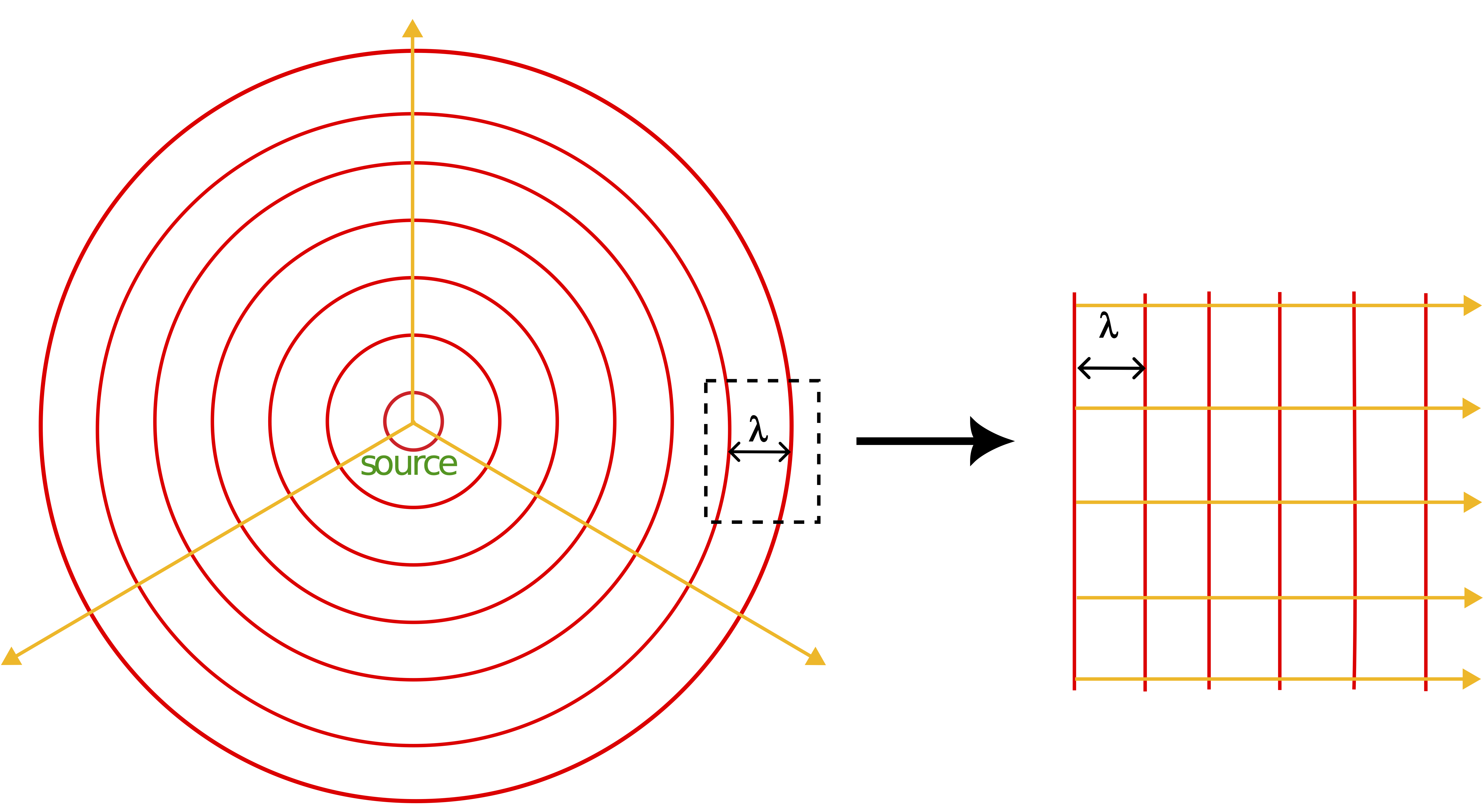
This approximation of multi-dimensional waves distant from the source is known as plane waves. Thus, the one-dimensional wave equation is often used to represent plane waves which originate from a source generating multi-dimensional waves. The distance between two neighboring crests is preserved to measure one wavelength.

Wave Intensity

In the previous section we mentioned that amplitude is only preserved in one-dimensional waves. This is assuming that dissipative effects of the medium are negligible. That is, the particles in the medium that oscillate do so without "friction." This means we are assuming that all of the energy in the wave remains within the wave, and none of the energy is converted into thermal energy in the medium. However, even neglecting friction amplitude no longer remains constant for multi-dimensional waves.

Consider now a wave radiating outward from a point source in two dimensions (think of a circular ripple on a pond caused by a pebble). Each position in the medium contains a particle oscillating harmonically (like a mass on a spring), and as the wave propagates outward, the number of oscillating particles increases. The particles in the medium are spaced the same everywhere, so the number of particles encountered by the circular wave is proportional to its circumference, and therefore proportional to its radius. This means that when the radius of the wave front doubles, it is oscillating twice as many particles in the medium. As the wave moves out, there is no energy lost, so when the circle enlarges, the energy is distributed amongst a larger number of oscillators. The energy in each oscillator is determined by its amplitude of oscillation, so for more oscillators to have the same energy as fewer oscillators, their amplitudes must decrease.

Figure 8.3.3: Circular Wave Energy Conservation

Let us see how the energy of the oscillator is related to amplitude. Recall, from 7A the total energy of a spring-mass system is the sum of kinetic and potential energy:

\[E_{\text{tot}}=KE+PE_{sm}=\dfrac{1}{2}mv^2+\dfrac{1}{2}kx^2\]

Amplitude is defined to be the maximum displacement from equilibrium (x=A), when the speed of the oscillator is zero (turnaround point). This results in the following expression for the total energy:

\[E_{\text{tot}}=\dfrac{1}{2}kA^2\]

Thus, the energy per oscillator is proportional to the square of the amplitude. This means that doubling the radius of the circle which doubles the number of oscillators between which this same energy is shared, the square of amplitude of each oscillation reduces by half, and the amplitude by a factor of \(\sqrt{2}\). Tripling the radius reduces the amplitude by a factor of \(\sqrt{3}\), and so on. In other words, amplitude is proportional to the inverse square-root of the radius:

\[A\propto \dfrac{1}{\sqrt{r}}\]

The figure above shows what happens to the amplitude of the wave in cross-section as it goes from a radius of 1 wavelength to 3 wavelengths.

The wave doesn't change its velocity from the inner circle to the outer circle, so the rate at which energy passes through each circle must be the same. What is different about two circles is the density of the energy contained in each. For the smaller circle, the energy is distributed over a smaller circumference than for the larger circle, so the energy density becomes smaller as the wave propagates outward, even though the total energy is constant. We can define power density in the same manner – by dividing the power of the wave (which is the same for both rings, and everywhere else) by the size of the region through which it is passing. This "power density" is called intensity. For our two-dimensional wave, this is the ratio of the power of the wave and the circumference of the circle through which it is passing:

\[I_{2d}\left(r\right) = \dfrac{P}{2\pi r} \]

Therefore, the intensity of a two-dimensional wave radiating outward from a central point varies in inverse proportion to the distance from the central source. We find that the intensity is proportional to the square of the amplitude:

\[A\propto \dfrac{1}{\sqrt{r}} \;\;\;\Rightarrow\;\;\;I\propto A^2\]

It turns out that the proportionality of intensity and square amplitude was the case for one-dimension as well. For a one-dimensional wave, the energy density does not change, because all of the energy is handed from one oscillator to another neighboring single oscillator. Therefore the power density (intensity) doesn't change, which is consistent with what we already know; the amplitude of a one-dimensional wave remains constant.

Far more common in our studies are three-dimensional waves with central sources (namely sound and light), and the power density in these cases involves dividing by a spherical surface area, rather than a circle. In this case, the intensity of the wave has units of watts per square meter (whereas the intensity of the two-dimensional wave had units of watts per meter), and we have:

\[I_{3d}\left(r\right) = \dfrac{P}{4\pi r^2} \]

Once again we find the same relationship between intensity and amplitude. The same mechanism is at work: as the wave moves outward from a central point, the number of oscillators on each spherical surface is proportional to the surface area. Doubling the radius of a spherical surface quadruples the surface area, so the number of oscillators grows with the square of the radius. This means that the energy per oscillator drops with the square of the radius, and the amplitude is inversely-proportional to the radius:

\[A\propto \dfrac{1}{r} \;\;\;\Rightarrow\;\;\;I\propto A^2\]

The relation between intensity and amplitude is therefore universal among waves, and one that we will keep in mind in the sections to come.