8.4: Doppler Effect

Stationary Source and Observer

Up to this point when we considered wave properties such as frequency, wavelength, and speed, we assumed that the source, which is generating the wave, and the observer, who is detecting the wave and measuring its properties, are both stationary. The animation below represents this situation where the central (red) dot is the source which flashes every time is emits a crest. The wave representation you see below is of a two-dimensional wave where the circles represent crests emanating out from the source, such as ripples in a pond. The distance between two consecutive circles is the wavelength of the wave. Since the representation below is an amination, you can also determine the period by timing how often the red dot flashes.

Figure 8.4.1: Source and Observer are Stationary

The blue dot to the left of the source is the observer which flashes every time that a crest passes through it. The idea of an observer is especially applicable to sounds waves, which we interpret directly in our daily lives. When the crests exert pressure on our ears, our eardrums vibrate. The amplitude of these vibrations is interpreted by our brains as loudness, and frequency of the vibrations is interpreted as the pitch of the sound. 

When both the source and the observer are stationary, the frequency according to both of them will be identical, as will be the wavelength (the measurement of the distance between two consecutive crests), and therefore the speed of the wave. The question we would like to ask next is what happens when there is motion involved of either the source, the observer, or both.

Moving Source

The animation below shows the source moving toward a stationary observer. This source, for example, could be an speeding ambulance which is emitting a loud sound of a specific pitch. If you watch the animation closely, the frequency with which the source is emitting is different the frequency with which the observer is receiving them, the blue dot (the observer) is flashing more frequently than the red dot (the source). How is it possible that the observer could be measuring a frequency different from what the source is emitting?  

Figure 8.4.2: Source Moving Toward Stationary Observer

Let us try to understand this phenomena from the perspective of the observer. It is apparent from the animation above, that the crests are more dense in front of the moving source and are less dense behind the source. Thus, the wavelength as measured by the observer in front of the moving source is shorter. When the source is stationary the distance between two consecutive crests is one source wavelength, \(\lambda_s\), the wavelength as measured by the source. However, when the source is moving, every time it emits a crest it moves a certain distance before emitting the next crest. Thus, it gets closer to the crest in front of it when it emits the next one, shortening the distance between two neighboring crests. Likewise, it gets further away from the crest behind it, lengthening the distance between crests behind the source. 

We can figure out this new distance between the crests by calculating the distance that the source moves between consecutive emissions of crests. The time it takes to emit two neighboring crests is one source period, \(T_s\), (period as measured by the source), the speed with which the source moves is source speed, \(v_s\), so the distance it moves is \(d=v_s T_s\). Thus, the new distance between two crests, which we call the observed wavelength, \(\lambda_o\), in front of the moving source is the source wavelength minus the distance the source moved in one period:

\[\lambda_o=\lambda_s-v_sT_s\label{L-doppler}\]

From this we can determine the frequency which the observer measures. We can use the relationships, \(\lambda=v/f\) and \(T=1/f\), to rewrite equation \ref{L-doppler} in terms of frequencies. We will leave the symbol, \(v\), without any subscript to mean the speed of sound. Notice, the speed of sound is the same for both the source and the observer in this scenario since it depends on the medium and the observer is stationary (you will see shortly how the speed of sound changes according to a moving observer). Replacing wavelength with frequency in Equation \ref{L-doppler} we get:

\[\dfrac{v}{f_o}=\dfrac{v}{f_s}-\dfrac{v_s}{f_s}\]

By rearranging the equation, we can express the observed frequency in terms of source frequency using the same method as above:

\[f_o=\dfrac{v}{v-v_s}f_s\label{toward}\]

You can see from the equation above that the observed frequency is larger than the source frequency when the source moves toward the observer, since the numerator, \(v\) is greater than the denominator, \(v-v_s\). This is consistent with the animation of the blue observer dot flashing at a greater frequency compared to the red source dot.

If the observer is standing behind the moving source instead, the animation shows that the crests get farther apart from a receding source. In this case, the source moves away from an emitted crest by a distance of \(v_sT_s\) before emitting the next crest. So the observed wavelength becomes: 

\[\lambda_o=\lambda_s+v_sT_s\]

Resulting in the following expression for the observed frequency:

\[f_o=\dfrac{v}{v+v_s}f_s\label{away}\]

In the equation above the observed frequency is lower than the source frequency, since the numerator, \(v\) is less than the denominator, \(v+v_s\). Since the speed of sound is fixed, the shorter wavelength in front of an approaching source results in a higher frequency, while the longer wavelength behind a receding source results in a lower frequency. Next time an ambulance is zooming by you, try to pay attending to the pitch of the siren as it approaches you and then recedes away from you. This phenomena is known as the Doppler effect.

Combing the two equations, the Doppler effect for a moving source can be written as:

\[f_o=\dfrac{v}{v\pm v_s}f_s\label{Doppler-source}\]

where the sign is a plus for a source moving away from the observer and a minus for a source moving toward the observer.

Moving Observer

Let us consider what happens when, instead of the source, the observer is moving toward or away from a stationary source. In this case since the source is stationary the distance between the crests is the same in front and behind the source, as shown in the animation of Figure 8.4.1. Thus, in this scenario the wavelength is fixed. A moving observer would measure the same distance between crests as it would if it was stationary. If the blue dot representing the observer moves toward the source in Figure 8.4.1, it would flash more frequently since it would encounter crests more often, than it would if stationary. Thus, the frequency according to the observe increases. But how is this possible if the wavelength remains the same and the medium does not change?

Let us think of this in terms of an analogy. Imagine you are driving in a vehicle with a train on tracks parallel to the road approaching you. The observer is you in the moving vehicle, and the train represents the moving wave. The distance between the cars of the train appears the same to you, so the wavelength is the same. But the frequency with which you are seeing each new car as you are moving in the opposite direction of the train is greater than if you were stationary. The train also appears to be moving faster than it does when you are stationary. Of course, the train itself is moving at a constant speed, but according to the observer the train is moving faster. If on the contrary you were moving in the same direction as the train, the train would appear to move slower, or even stationary if your speed is identical to that of the train. This is known as relative motion, the speed of objects depends on the frame from which they are measured. A stationary observer will measure the train moving at a different speed from the observer in a moving vehicle.

Therefore, when the observer is moving toward the source emitting a wave, the speed of sound appears to increase. It does so according to this equation, \(v+v_o\), where \(v\) the speed of sound according to the rest frame, and \(v_o\) the speed of the observer. Thus, the frequency as measured by the observer is the speed of sound according to the observer dividing by the wavelength emitted by the source:

\[f_o=\dfrac{v+v_o}{\lambda}=\dfrac{v+v_o}{v}f_s\label{o-toward}\]

where we used \(\lambda=v/f_s\) for the wavelength. If the observer is moving away from the source, or analogously you are driving in the same direction as the moving train, then the speed measured by observer decreases, and the speed of sound according to the observer becomes \(v-v_o\). Using the same reasoning as in Equation \ref{o-toward} the observed frequency for an observer moving away from the stationary source is:

\[f_o=\dfrac{v-v_o}{v}f_s\label{o-away}\]

Combing the two equations, the Doppler effect for a moving observer and a stationary source is:

\[f_o=\dfrac{v\pm v_o}{v}f_s\label{Doppler-ob}\]

The observed frequency is higher than the source one when the numerator is bigger than the denominator, which is the case when the sign is positive. This is consistent with the observation of the blue dot flashing more frequently if it was to move toward the source. On the contrary, we choose a negative sign when the observer is moving away from the source, resulting in a lower observed frequency.

Combined Doppler Effect

For completeness, let us consider the Doppler effect when both the source and the observer are moving. When both are moving, the observe measures a different speed of sound due to relative motion and a different wavelength due to source moving. Thus, the speed of sound measured by the observer is \(v\pm v_o\) (depending on direction of motion) and the wavelength is \(\lambda_o\). Thus, we get the following expression for the frequency:

\[f_o=\dfrac{v\pm v_o}{\lambda_o}\]

The wavelength that the observer measures is the same as calculated for a moving source. Using the result in Equation \ref{Doppler-source}, we get a general expression for the combined Doppler effect:

\[f_o=\dfrac{v\pm v_o}{v\mp v_s}f_s\label{Doppler}\]

You can see from the equation above that when the observer is not moving, \(v_o=0\), we recover Equation \ref{Doppler-source} for the stationary observer and a moving source. When the source is stationary, \(v_s=0\), then we obtain Equation \ref{Doppler-ob} for a stationary source and a moving observer. Naturally, if both are stationary, there is no Doppler effect resulting in \(f_o=f_s\).

Since there are many parameters to keep track of when solving problems which involve the Doppler effect, here is a summary of all the terms in Equation \ref{Doppler}:

• Observed frequency, \(f_o\), frequency as measured by the observer.
• Source frequency, \(f_s\), frequency as emitted by the source.
• Wave speed, \(v\), is the speed of the wave as determined by the medium, most commonly applied to the speed of sound in air.
• Speed of the observer, \(v_o\), use a plus sign in the numerator when the observer is moving toward the source and a minus sign when the observer is moving away from the source.
• Speed of the source, \(v_s\), use a minus sign in the denominator when the source is moving toward the observer and a plus sign when the source is moving away from the observer.

Sound waves are not the only types of waves which exhibit the Doppler effect. In fact, the Doppler effect which was first described by an Austrian mathematician and physicist Christian Doppler in 1842 due to his observations of light coming from distant stars. The Doppler effect eventually led to the idea of an expanding universe, since it was observed that the light coming from distant stars always seems to be redshifted, meaning that the wavelengths of light emitted from the stars are longer than expected. This implies that the stars around us are always receding or moving away, consistent with a notion of an expanding universe. Even though, similar principles apply to light as to sound, since electromagnetic waves move at the speed of light, Doppler effect described by Equation \ref{Doppler} no longer applies. One needs to consider relativistic effects to calculate the Doppler effect. 

There are also multiple applications of the Doppler effect in medicine, specifically in ultrasound technology. You will explore a model of ultrasound technology in Example 8.4.2 below. Police radars use the Doppler effect to calculate the speed of moving vehicles. The radar emits a wave, which then is reflected from the moving vehicle, and is detected by the radar. However, since radars emit electromagnetic waves, such as radio waves, relativistic Doppler effect equations need to be used.

Example \(\PageIndex{1}\)

You are sitting in your car and you hear an ambulance which is moving toward you emitting a loud sound at a set frequency. Then you start moving in the same direction and at the same speed as the moving ambulance. Once you are moving you hear the frequency of the siren as 9/10 the frequency than you heard when you were stationary. Use the speed of sound as 344 m/s. Determine your speed.

Solution

When both you are the ambulance are moving in the same direction, the ambulance is moving toward you (so the sign in the denominator of the Doppler equation is negative) and the observer (you in the car) is moving away from the ambulance (so the sign in the numerator of the Doppler equation is also negative). Since both the car (the observer) and the ambulance (the source) are moving at the same speed, then \(v_o=v_s\). Plugging this into the Doppler equation:

\[f_o=\dfrac{v-v_o}{v-v_s}f_s=\dfrac{v-v_o}{v-v_o}f_s=f_s\nonumber\]

Thus, when the observer and the source are moving in the same direction and with the equal speed, there is no Doppler shift. To visualize this, think of driving on the highway right next to a car which is moving at the same speeds as you. That car appears to be stationary. Thus, when both the source and the observer are moving identically relative to each other, it is equivalent to both being stationary, resulting in no Doppler shift of frequency. Therefore, the source frequency (equivalent to the frequency the car observes when moving) is 9/10 the frequency the car observed when stationary, \(f_o\):

\[f_s=\dfrac{9}{10}f_o\nonumber\]

The ambulance is moving toward the car, so it observed a higher frequency when stationary. The Doppler equation for the scenario of a source moving toward a stationary observer is:

\[f_o=\dfrac{v}{v-v_s}f_s\nonumber\]

Using the information of the ratio between the observed and source frequencies we get:

\[\dfrac{10}{9}=\dfrac{v}{v-v_s}\nonumber\]

Solving for the speed of the source with some algebraic manipulations we obtain the following speed of the source:

\[v_s=\dfrac{v}{10}=\dfrac{344 m/s}{10}=34.4 m/s\nonumber\]

The above result is equivalent to the speed of the car once it starts moving as stated in the problem.

Example \(\PageIndex{2}\)

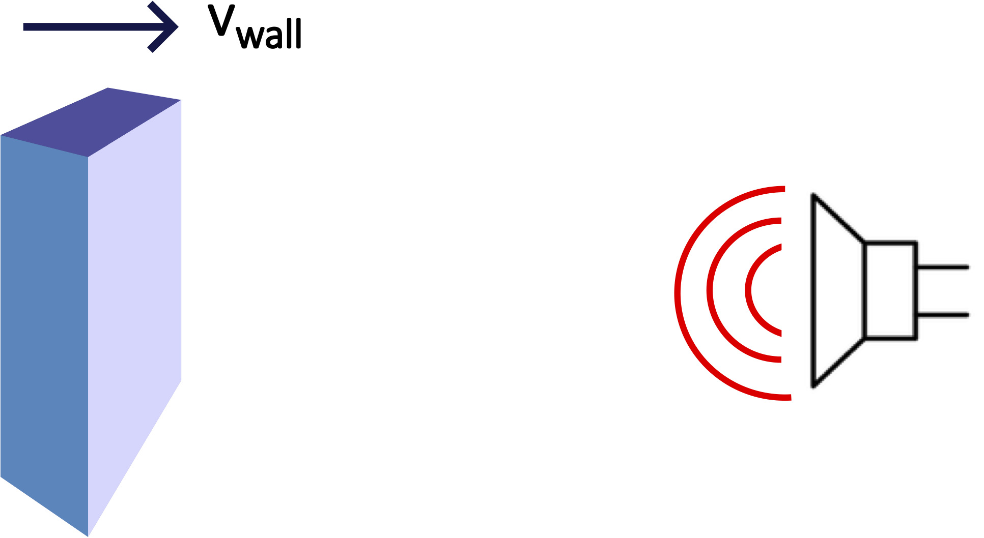
Ultrasound technology uses the principle of Doppler effect to calculate the speed of blood in human veins. A sound wave generated by the ultrasound machine reflects off the moving blood cells and is then detected by the ultrasound machine. For simplicity, let us mimic this situation with a stationary sound source (a speaker replacing the ultrasound machine) and a wall moving toward the source (the wall replacing the moving blood), as seen below. Assume the source is emitting a frequency of 200 Hz, and the wall is moving with 5 m/s. Use the speed of sound in air as 344 m/s. Calculate the frequency of the sound that comes back to the source after the sound was reflected from the moving wall. Hint: you need to use the Doppler effect twice, once for the outgoing wave, and once for the reflected one.

Solution

When the wave is first emitted, the moving wall acts as an observer of this wave. It detects the frequency of this wave which can be calculated according to the equation of a moving observer toward a stationary source:

\[f_o=\dfrac{v+v_{\text{wall}}}{v}f_s\nonumber\]

Once the wave is reflected, now the source detects that wave. The wall becomes the source of the wave, since it is now emitted the reflected wave. The new source frequency is then the observed frequency from the equation above. Using the Doppler effect equation for a moving source toward a stationary observer, the frequency of the reflected wave as detected  by the original source is:

\[f_o=\dfrac{v}{v-v_s}f_s\nonumber\]

The speed \(v_s\) is the speed of the wall, \(v_{\text{wall}}\), and \(f_s\) is the frequency observed by the wall from the source as given in the first equation. Combining these results we get:

\[f_o=\dfrac{v}{v-v_{\text{wall}}}\cdot \dfrac{v+v_{\text{wall}}}{v}f_s=\dfrac{v+v_{\text{wall}}}{v-v_{\text{wall}}}f_s\nonumber\]

Plugging in the given numerical values, we obtain the frequency of the reflected wave as detected by the source:

\[f_o=\Big(\dfrac{344+5}{344 -5}\Big)(200 Hz)=205.9 Hz\nonumber\]