8.2: Wave Representation

Simple Harmonic Motion

For the rest of the course we will focus on infinite repeating waves of a specific type, harmonic waves, whose properties were described in the previous section. We saw how to represent the wave graphically and defined some important wave properties. In this section we want to write down a mathematical expression for one-dimensional harmonic waves and make connections between the mathematical and graphical wave representations. 

In order to represent the wave mathematically, let us start by thinking of one oscillator in the medium. We discussed in the previous section that when a wave propagate through a medium, the motion of each particle in the medium can be treated as an oscillator around the equilibrium position of the medium. When the wave is harmonic, these oscillations can be described by a simple harmonic oscillator, similar to the spring-mass system you studied in 7A as depicted in the figure below.

Figure 8.2.1: Simple Harmonic Oscillator

In 7A we focused on describing the energy of the harmonic oscillator: the potential and kinetic energy relative to the equilibrium position. Now we want to focus on the dynamics of the harmonic oscillator, in order to describe how the position of the oscillator changes with time. This result can be obtained by using Newton's second law and the force for a simple harmonic oscillator introduced in 7A in Section 2.5. Hooke's Law describes the restoring force for simple harmonic motion:

\[F_{net}=-ky\]

where \(k\) is the spring-constant, and \(y\) is displacement from equilibrium. Combining Hooke's Law with Newton's second law we get:

  \[F_{net}=ma=-ky\]

Using the definition of acceleration and rewriting the above equation such that it is solvable for position as a function of time, we get:

\[m\dfrac{d^2y}{dt^2}+ky=0\label{DE}\]

From the above equation we can see that \(y\) has to be represented by a function that when differentiated twice it returns to the negative of same function. The functions that have this property are sinusoidal, either sine or cosine. As a result the posltion of a harmonic oscillation as a function of time can be represented as:

\[y(t)=A\sin\Big(\omega t+\phi_o\Big)\label{SHO}\]

where \(\omega=\sqrt{k/m}\) (you will show this result in the Example 8.2.1 below). It is reasonable that harmonic motion which is periodic is represented by a sine function which repeats. The amplitude, \(A\), is the maximum displacement, since the sine function can at most be equal to one. For the spring-mass system the amplitude represents the distance that you initially pulled the spring-mass away from equilibrium before releasing it. We learned from 7A that due to conservation of energy the spring-mass displacement cannot be bigger than the distance from which it is released. 

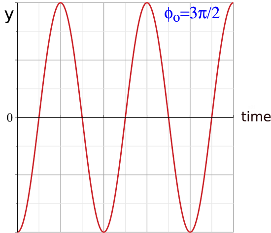
The value \(\phi_o\) inside the sine function is a constant which determines the initial displacement (at t=0 sec) of the system. For example, if you pulled the spring-mass down and released it, such that the displacement is \(y=-A\) at \(t=0\) sec, then:

\[y(0)=-A=A\sin(\phi_o)~~\Rightarrow~~\sin(\phi_o)=-1~~\Rightarrow~~\phi_o=\dfrac{3\pi}{2}\]

The sine function in Equation \ref{SHO} for the above value of \(\phi_o=3\pi/2\) is plotted below, starting from a maximum displacement below equilibrium.

Figure 8.2.2: Phase Constant Example

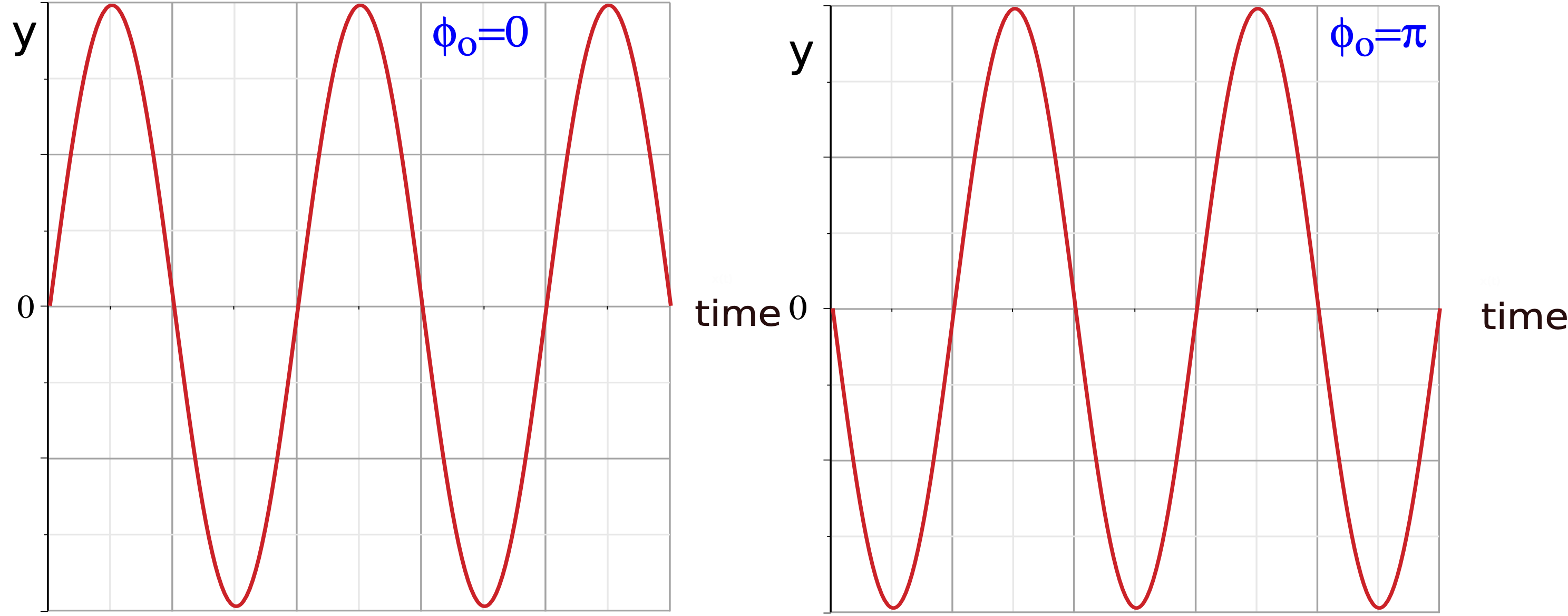
In another example, if you define the initial conditions (t=0s) at the time the spring-mass passes equilibrium (y=0), then:

\[y(0)=0=A\sin(\phi_o)\]

The above scenario is more complicated, since there are two solutions in one cycle of the sine function for this initial scenario, \(\phi_o=0\) or \(\phi_o=\pi\). These phase constants correspond to two physical situations that are possible within one cycle when the mass is at equilibrium. If the mass is vertical as in Figure 8.2.1, it could either be moving down or up as it passes equilibrium. In the figure below it can be seen that a starting position of the spring-mass at equilibrium moving up corresponds to \(\phi_o=0\), while the spring-mass moving down at equilibrium at t=0 sec results in \(\phi_o=\pi\), the left figure is shifted by half a cycle to obtain the right figure.

Figure 8.2.2: Phase Constant

 

By definition of one period \(T\) introduced in Section 8.1, the function should return to its original position after one cycle. For trigonometric functions a convenient unit for counting cycles is radians. Radians of \(2\pi\) represent one cycle, such that:

\[sin(x+2\pi)=sin(x)\label{sin}\]

 To assure that the quantity inside the sine function is in units of radians, Equation \ref{SHO} can be written as:

\[x(t)=A\sin\Big(\dfrac{2\pi}{T}t+\phi_o\Big)\label{time-dep}\]

where \(\omega\) Equation \ref{SHO} is written in terms of \(2\pi/T\). To check that this expression is consistent with the definition of one period, the function should be identical when one period of time passes, \(t\rightarrow t+T\):

\[y(t+T)=A\sin\Big(\dfrac{2\pi}{T}(t+T)+\phi_o\Big)=A\sin\Big(\dfrac{2\pi}{T}t+2\pi+\phi_o\Big)=A\sin\Big(\dfrac{2\pi}{T}t+\phi_o\Big)=y(t)\label{time}\]

In the above equation we used the property of the sine function given in Equation \ref{sin}.

Example \(\PageIndex{1}\)

Show that that \(\omega=\sqrt{k/m}\) using Equation \ref{DE} and Equations \ref{SHO}.

Solution

Starting with Equation \ref{SHO}:

\[y(t)=A\sin\Big(\omega t+\phi_o\Big)\nonumber\]

Differentiating it once:

\[\dfrac{dy}{dt}=A\omega\cos(\omega t+\phi_o)\nonumber\]

Now differentiating it again:

\[\dfrac{d^2y}{dt^2}=-A\omega^2\sin(\omega t+\phi_o)\nonumber\]

Now plugging the above results into Equation \ref{DE}:

\[-A\omega^2m\sin(\omega t+\phi_o)+kA\sin(\omega t+\phi_o)=0\nonumber\]

Cancelling the sine terms and the amplitude:

\[-\omega^2m+k=0\nonumber\]

Solving for \(\omega\):

\[\omega=\sqrt{\dfrac{k}{m}}\nonumber\]

Harmonic Wave Equation

The discussion above which led to Equation \ref{time-dep} does not capture the full wave phenomena since it only describes the motion of one oscillator at fixed position in the medium as a function of time. That "fixed position" refers to the location in the medium about which the particle oscillates. To describe the wave fully, we also need to incorporate the wave motion in space throughout the medium. In other words, we want to write down a mathematical expression describes the displacement of all the oscillators in the medium at all times. A one-dimensional harmonic wave can be expressed mathematically as:

\[y(x,t) - y_o = A \sin{\left(\dfrac{2\pi}{T}t \pm \dfrac{2\pi}{\lambda}x + \phi_o \right)}\label{wave-equation}\]

The displacement away from equilibrium at position \(x\) and time \(t\) is given by the left-hand side, \(y(x,t) - y_o\), where \(y_o\) is equilibrium position, and \(y(x,t)\) is the oscillator's position relative to some chosen zero. In most cases it is convenient to set \(y_o=0\), since this will result in a symmetric displacement about the x-axis with the maximum displacement at \(A\) and the minimum displacement at \(-A\). But when the equilibrium position is not set to zero, then the entire sine function shifts vertically either up or down by the chosen value of \(y_o\).

Equation \ref{time-dep} demonstrated that for a single harmonic oscillator the sine function has identical form after a time of one period. The second term in Equation \ref{wave-equation}, which describes the spatial periodicity of the wave, resembles the first term very closely. Using the same method as in Equation \ref{time}, one can show that the wave equation is identical after the value \(x\) increases by any multiple of wavelength. 

The fixed phase constant \(\phi_o\) is different from the one in Equation \ref{time-dep}, since it describes what the wave looks like both at the initial time, \(t=0\), and at a location defined as zero, the origin \(x=0\). For example, assume that there is a crest at \(x=0\) and \(t=0.\) If we set the equilibrium at zero (\(y_o=0)\), then the initial displacement of the wave is equal to \(A\), since it is a crest:

\[y(0,0)=A = A \sin(\phi_o)~~\Rightarrow~~ \sin(\phi_o)=1 ~~\Rightarrow ~~ \phi_o=\dfrac{\pi}{2}\label{phio-crest}\]

The symbol \(\pm\) asks us to choose the sign of either \(+\) or \(-\) depending on the direction that the wave travels. How do we determine the appropriate sign when the wave is moving to the right (values of \(x\) are increasing) or when the wave is moving to the left (values of \(x\) are decreasing)? The quantity \(y(x,t)\) gives the displacement of a particular part of the wave as it travels through space and time. So if you are watching a particular part of the wave, the displacement should stay fixed for all values of position and time. Let's say you start watching a crest at \(t=0\) of a wave that starts at \(x=0\) and moves to the right. If you watch the crest for a time span of a quarter of a period, \(t=T/4\), then this crest must be at a position quarter of cycle in the direction of increasing x, \(x=\lambda/4\). Using the result in Equation \ref{phio-crest} for the phase constant when the initial conditions of the wave is a crest, the displacement at a time \(t=T/4\) is:

\[y\Big(\dfrac{\lambda}{4},\dfrac{T}{4}\Big )=  A \sin{\left(\dfrac{2\pi}{T}\cdot\dfrac{T}{4} \pm \dfrac{2\pi}{\lambda}\cdot\dfrac{\lambda}{4} +\dfrac{\pi}{2} \right)}= A \sin{\left(\dfrac{\pi}{2}\pm \dfrac{\pi}{2} +\dfrac{\pi}{2} \right)}=\begin{cases} + \Rightarrow& A\sin\Big(\dfrac{3\pi}{2}\Big)=-A\\ - \Rightarrow & A\sin\Big(\dfrac{\pi}{2}\Big)=A \end{cases}\]

Since you were tracking a crest, the correct sign to choose is negative since it resulted in a displacement equal to A, according to the above equation. If the wave was moving to the left instead, then its position a quarter period later would be at \(x=-\lambda/4\), and following the same steps are outline above you would find that a positive sign in front of the spatial term would give the correct result. To summarize, we choose a "\(+\)" sign for left-moving waves and a "\(-\)" sign for right-moving waves when writing down the wave equation given in Equation \ref{wave-equation}. 

There is another very useful quantity which we will often use to describe wave properties. The total phase, \(\Phi\), (not to be confused with the fixed phase constant \(\phi_o\)) is defined as the quantity inside the sine function of the wave equation:

\[\Phi (x,t) \equiv 2 \pi \dfrac{t}{T} \pm 2 \pi \dfrac{x}{\lambda} + \phi_o \]

The total phase identifies a particular point on a wave. When we imagine ourselves riding the wave, or when we watch a wave crest or trough travel, we are really following a point of constant total phase. Going back to the direction discussion, since the total phase of any part of the wave must remain constant, if the wave is moving to the right (time and position are both increasing), the sign in front of the spatial term must be negative to keep \(\Phi\) constant. On the contrary, if the wave is moving to the left (time is increasing while position is decreasing), then the sign must be positive to keep the total phase fixed.

Since the wave equation has many terms, it is worthwhile noting the difference between variables and parameters, and the dependence of parameters on the source of the wave or the medium through which it travels:

• The parameters \(A, T, \lambda , \phi_o , y_o\) and the choice of \(+\) or \(-\) are constants for any given harmonic wave. They describe the wave and its behavior. The period and the amplitude are determined by the source of the wave. The phase constant, the equilibrium position, and the direction is determined by the choice of origin and coordinate system, but remain fixed once they are established. The wave speed is determined by the medium. The wavelength depend on both the period and the wave speed.
• The variables (for any \(x\) and any \(t\)) describe the all the space and time in which the wave exists. These variables determine the displacement of the medium at that particular time and location.
• We can ask about the displacement at different locations and times by changing variables, but parameters for a wave are fixed values.

Now that we have an equation to fully describe one-dimensional wave phenomena, we want to see if it is possible to represent it graphically. Typically, you can plot some behavior by taking the equation which it describes and plotting it as a function of the variable. But for the wave equation there are two variables, space and time. So, you can fix a particular time and make a plot of the wave as a function of position, which we called the snapshot plot in the previous section, which does not contain any temporal information about the wave. Or you can look at the medium at a specific location (fix the position) and plot how that part of the medium oscillate with time, but then you loose the spatial characteristics of the wave. Thus, it is clear that need more than one plot to fully describe wave phenomena. But are only two plots enough to describe the wave all all positions and all instances of time? Let us start by analyzing the two plots shown below.

Figure 8.2.3: Graphical Representation of a Wave

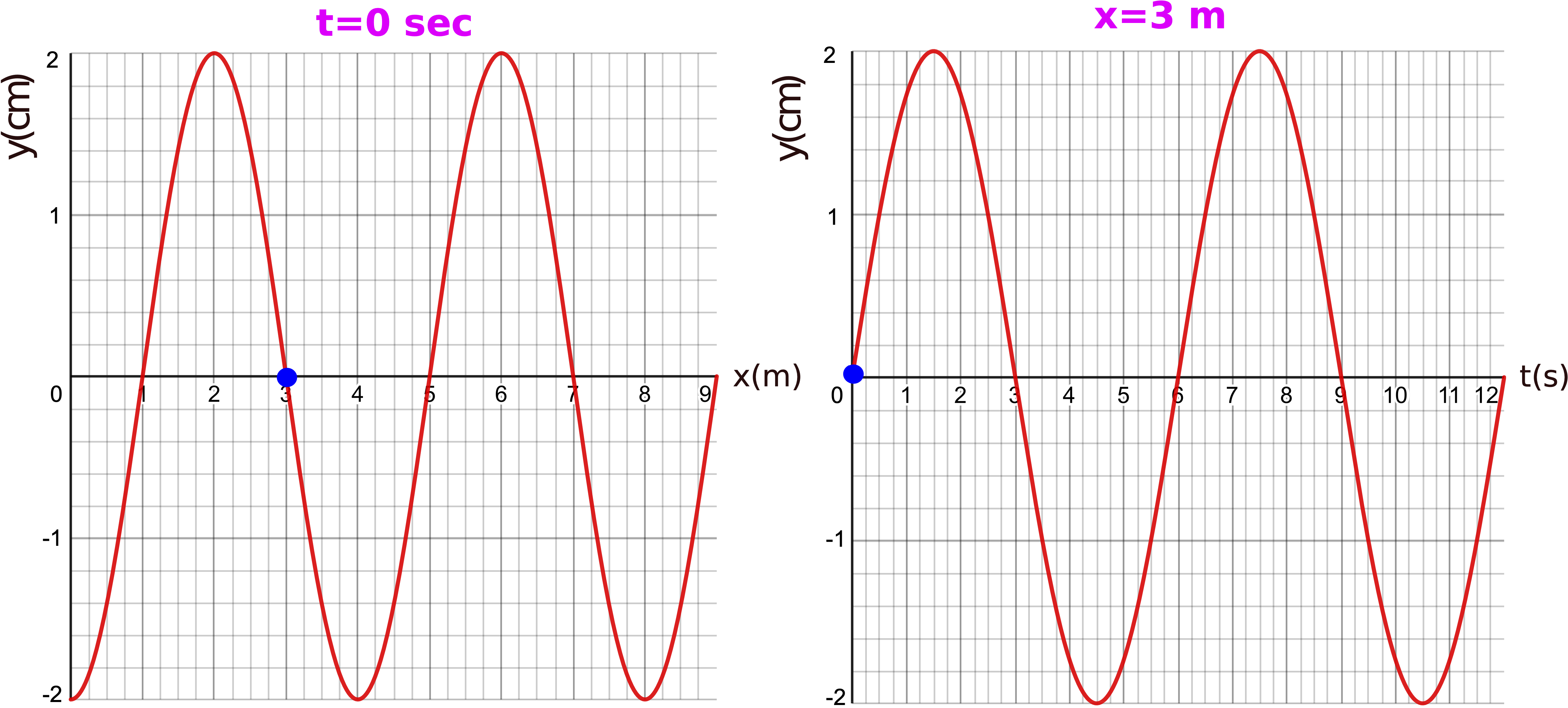
The plot on the left is a snapshot plot of the wave taken at \(t=0\) sec. You can read from the plot the amplitude of the wave, \(A=2\) cm, and the wavelength, \(\lambda=4\) m. The plot on the right show the oscillation of the medium at \(x=3\) m as a function of time. It shows the same amplitude which has to be consistent between the two plots. The plot also provides information about the period, \(T=6\) s. From both plots we can see that the equilibrium is set at zero, \(y_o=0\). 

To fully write down the wave equation, we still need to figure out the wave direction and the fixed phase constant. Let us think about direction first. We are given a snapshot (a paused "movie" of the moving wave) a \(t=0\) sec. We want to figure out whether we have enough information from the two plot which will allow us to determine if the wave will shift to the right or the left as some later time, when we un-pause the "movie". The only additional information we do have is the displacement at \(x=3\) m position will increase after \(t=0\) sec, or a crest is moving toward the \(x=3\) m location. The two (blue) dots shown in Figure 8.2.3 represent the same position and time (\(t=0\) s and \(x=3\) m). In other words, the two dots are the common point between the two plots, which happens to be an equilibrium displacement. Since the right plot tells us that the displacement at \(x=3\) m will increase after \(t=0\) s, shifting the snapshot plot in the correct direction of motion should give the same result. Since we want a crest to approach the \(x=3\) m position, then the snapshot plot needs to be shifted to the right.  Figure 8.2.4 below stresses this point by plotting the shifted snapshot at a later time of 0.5 seconds. 

Figure 8.2.4: Shifting the Snapshot Plot

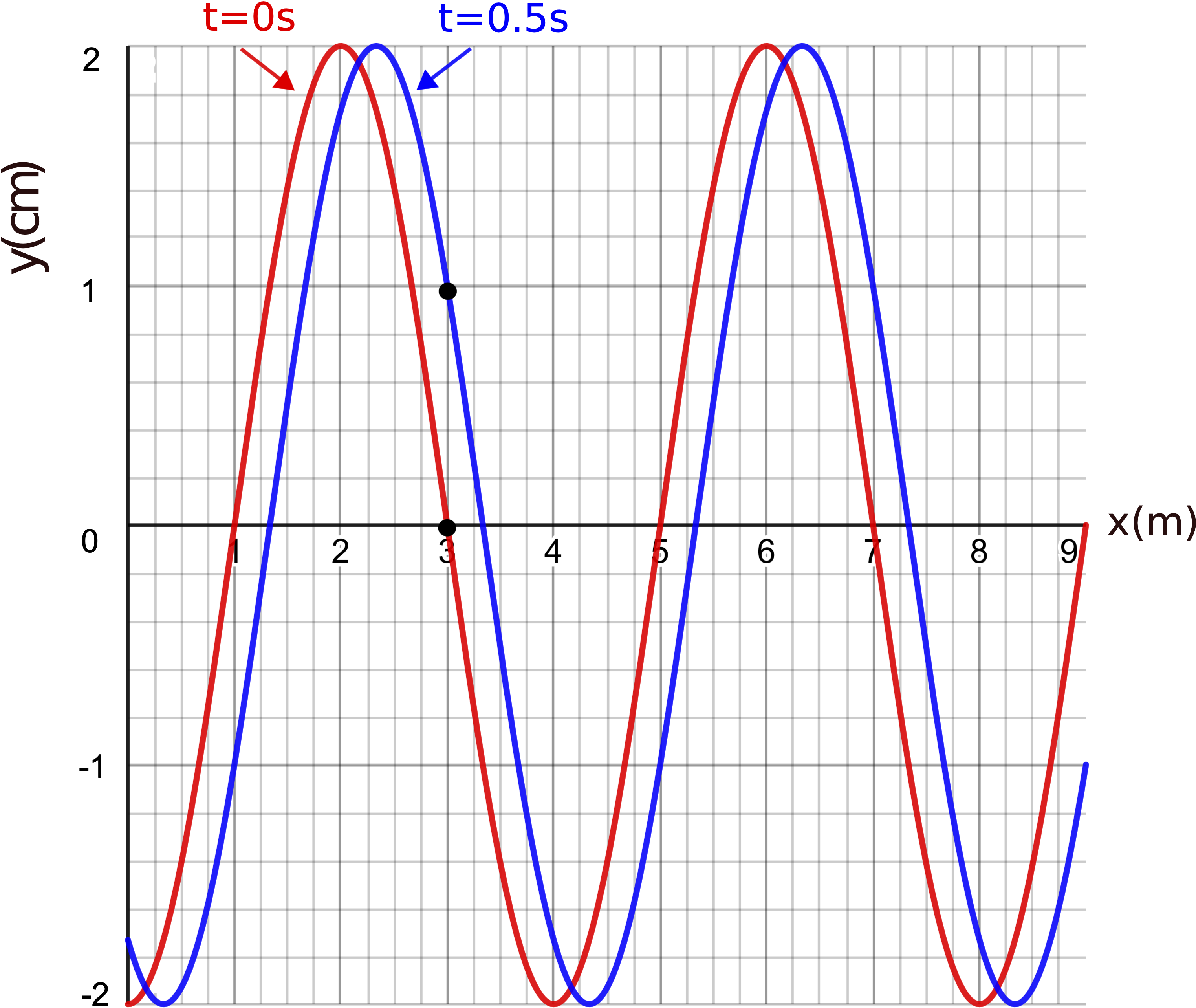
The time plot in Figure 8.2.3 shows that at \(t=0.5\) s the displacement at x=3m is going to be around 1 cm. The time of 0.5 seconds is 1/12 of one cycle since one cycle is 6 seconds. This corresponds to the wave moving by 1/12 of one wavelength or 1/3 m, which can be approximately seen by the difference in the two overlapping plots in the figure above. After the shift, the displacement at x=3m went up to 1 cm, as expected. If you were to shift the plot to the left instead, then the displacement would decrease, which is not consistent with the time-dependent plot. Therefore, we conclude that this wave is moving to the right.

Lastly, let's see if it is possible to obtain the fixed phase constant from these two plots. We defined \(\phi_o\) as the displacement of the wave at \(t=0\) s and \(x=0\) m. From the snapshot in Figure 8.2.3 you can see that this value corresponds to a trough. Plugging this into Equation \ref{wave-equation} we get:

\[y(0,0)=-2cm=(2cm)\sin(\phi_o)\Rightarrow \sin(\phi_o)=-1 \Rightarrow \phi_o=\dfrac{3\pi}{2}\label{Ex-phio}\]

This was of phase constant was simply to obtain. However, not all values of fixed phase constant could be easily read from the plot. For example, a fixed phase constant of \(\pi/4\) corresponds to displacement of 0.7071 (if amplitude is one), which would be hard to interpret from the plot. But there is no need to only use the values at the origin and initial time. You can use any point on the plot and just solve for the phase constant. For example, from the snapshot plot in  Figure 8.2.3, we can see that at \(x=2\) m, the displacement is a crest. Since the snapshot plot is at \(t=0\) sec, plugging into the wave equation, and using the parameters which were already determined we get:

\[y(x=2m,t=0s) = 2cm=(2cm) \sin{\left(\dfrac{2\pi}{6s}(0) - \dfrac{2\pi}{4m}(2m) + \phi_o \right)}=(2cm)\sin(-\pi+\phi_o)\Rightarrow \sin(-\pi+\phi_o)=1\]

The total phase has to be equal to \(\pi/2\) for a crest, since \(\sin(\pi/2)=1\). Therefore, solving for the phase constant we get:

\[-\pi+\phi_o=\dfrac{\pi}{2}\Rightarrow \phi_o=\dfrac{3\pi}{2}\]

which gives a result identical to the one found in Equation \ref{Ex-phio}. You can choose any other location from the two plots, and you will get the same result for the fixed phase constant. In general, it is always helpful to choose either a crest or a trough to solve for \(\phi_o\), since there is only one value for the total phase, \(\pi/2\) for crests and \(3\pi/2\) for troughs. You can also use an equilibrium value but there are two solution for the total phase, 0 or \(\pi\), so you would need to decide which one is the correct result, depending on how the function is changing after the equilibrium location that you chose. Any other value except for the equilibrium, a crest, or a trough may be difficult to read from the plot.

There are infinite number of solutions for the fixed phase constant, since you can also add or subtract any multiple of \(2\pi\) to the phase constant and obtain the same result for the wave equation. For example, another possible solution for the phase constant in Equation \ref{Ex-phio} is \(-\pi/2\) or \(7\pi/2\) or even \(23\pi/2\). In fact, if you were to choose another crest or trough to work with, you might obtain a number different from \(3\pi/2\). In general, for simplicity it is best to keep the value of phase constant between \(-\pi\) and \(\pi\).

Putting everything together the wave equation for the wave depicted in Figure 8.2.3 is:

\[y(x,t)=(2cm)\sin{\left(\dfrac{2\pi}{6s}t - \dfrac{2\pi}{4m}x +\dfrac{3\pi}{2}\right)}\]

Note, it is important to write units for the parameters such as amplitude, wavelength, and period to make sure that correct units are used when plugging values into \(x\) and \(t\) and solving for \(y(x,t)\).

Example \(\PageIndex{2}\)

Two buoys are oscillating up and down as ripples in a pond continuously pass through them. At t=6 sec you observe that the buoy which is at position x=4 m is at equilibrium, and the second buoy at position x=30 m is at a trough. You also count three crests and three troughs between the two buoys at t=6 sec. The vertical distance between the two buoys at t=6 sec is 0.2 m. The frequency of the wave is 0.5 Hz.

a) Calculate the speed of the wave.

b) At t=6.5 sec the buoy which is at x=4 m is found at a crest. Is the wave moving to the right or the left? 

c) Write down the full wave equation for this wave.

Solution

a) To find the speed we are missing direct information about the wavelength of the wave. It is helpful to visualize this problem by making a picture of the two buoys at t=6 sec. The x=4m buoy is at equilibrium and the x=30m buoy is at a trough, and there are 3 crests and troughs in between them. 

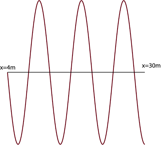
From the picture we see that there are three and one quarter cycles between these points which gives direct information about the wavelength:

\[3.25\lambda=(30-4)m\nonumber\]

\[\lambda=\dfrac{26m}{3.25}=8 m\nonumber\]

Using the given frequency, we can calculate the speed of the wave:

\[v=\lambda f=(8 m)(0.5 Hz)= 4 m/s\nonumber\]

b) From 6 seconds to 6.5 seconds, 0.5 seconds passed. The period is \(T=1/f=2 s\), so 0.5 sec is one quarter of a cycle. There is a crest one quarter cycle to the left of the buoy at x=4m (see picture above), so the wave is moving to the right.

c) Since the vertical distance between the two buoys is the distance between equilibrium and a minimum displacement, the amplitude is 0.2 m. The last parameter left to determine is the phase constant.  It is simplest to choose a crest or a trough at a specific time and location. From the picture above, let us use the crest at 10m, which is a three quarters of a wavelength to the right of the buoy at x=4m. Plugging into the wave equation:

\[y(x=10 m,t=6 s) = (0.2m)\sin{\left(\dfrac{2\pi}{2 s}\cdot 6 s - \dfrac{2\pi}{8m}\cdot 10m + \phi_o \right)}=0.2m\nonumber\]

Which results in the total phase being equal to \(\pi/2\):

\[6\pi-\dfrac{5\pi}{2}+\phi_o=\dfrac{\pi}{2}\Rightarrow \phi_o=-3\pi \nonumber\]

Note, although mathematically the result for the fixed phase constant came to \(-3\pi\), this is equivalent to \(\pi\) due to the sine function property that changing the phase by any multiple of \(2\pi\) does not change the sine function. And it is always more presentable to express the fixed phase constant with a value between \(-\pi\) and \(\pi\), although it is not technically wrong to leave it outside this range. So we choose:

\[\phi_o= \pi\nonumber\]

Combining all the results, the wave equation for this wave is:

\[y(x,t) = (0.2m)\sin{\left(\dfrac{2\pi}{2 s}t - \dfrac{2\pi}{8m}x + \pi \right)}\nonumber\]

Example \(\PageIndex{3}\)

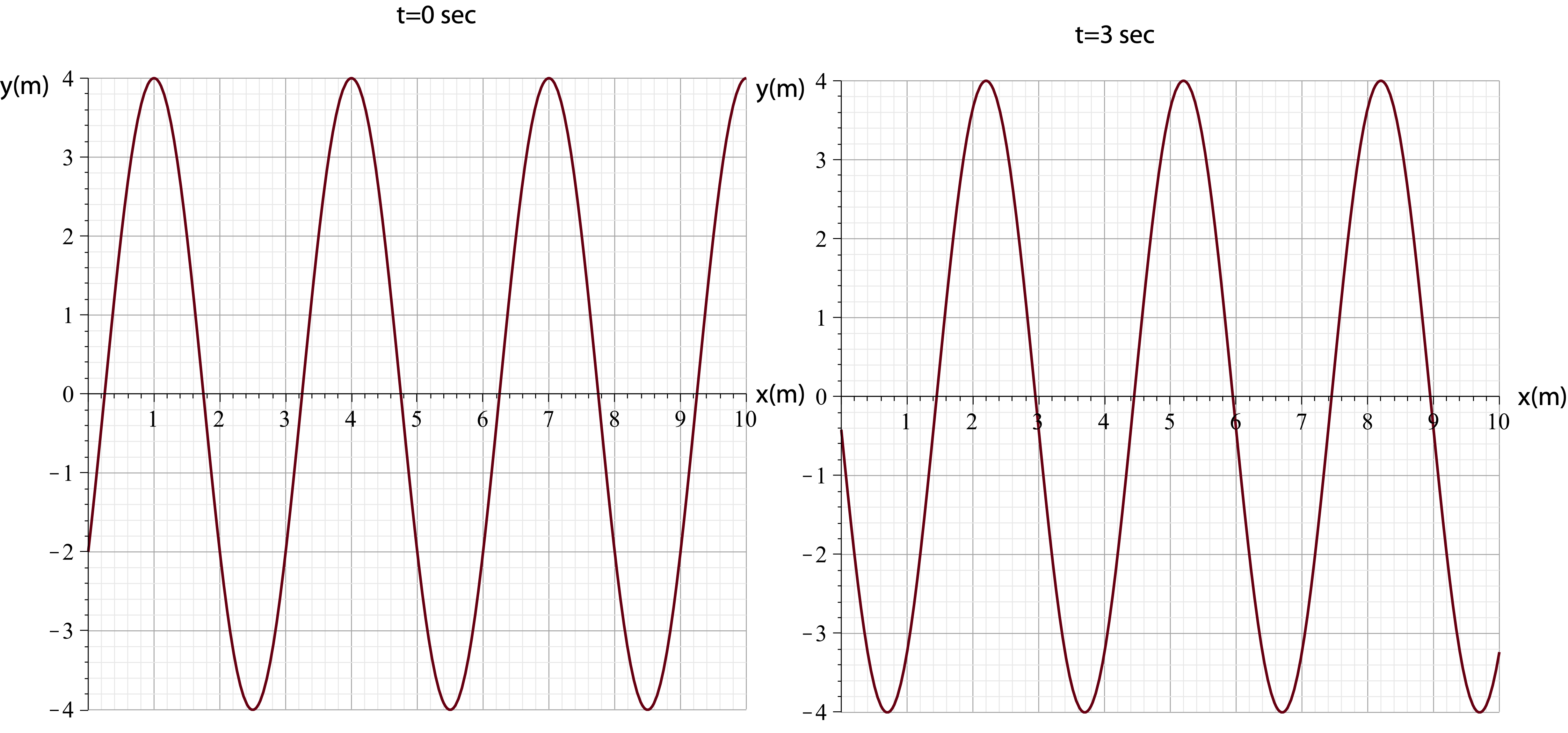
You are enjoying spring break at the ocean but decide to prepare for 7C by analyzing ocean waves. You take pictures of the waves 3 seconds apart and make two plots of wave displacement over 10 meters. You also note that the crest in at x=7 m and t=0 sec is the same crest as the one at x=5.2 m and t=3 sec. Write down the wave equation for this wave.

Solution

The wave moves to the left since the crest moves in the negative x-direction (from 7m to 5.2m) as time moves forward. The crest moves 1.8 meters in 3 second, so the wave speed is: 

\[v=\dfrac{d}{t}=\dfrac{1.8 m}{3 s}= 0.6 m/s\nonumber\]  

The wavelength is 3 meters from the plots. Solving for period:

\[T=\dfrac{\lambda}{v}=\dfrac{3 m}{0.6 m/s}=5 s\nonumber\]

Let us use the crest at t=0sec and x=1m to find the phase constant:

\[y(x=1 m,t=0 s) = (4 cm)\sin{\left(\dfrac{2\pi}{5 s}\cdot 0  + \dfrac{2\pi}{3 m}\cdot 1m + \phi_o \right)}\nonumber\]

Since it is a crest:

\[\dfrac{2\pi}{3}+\phi_o=\dfrac{\pi}{2}\nonumber\]

Resulting in: 

\[\phi_o= -\dfrac{\pi}{6}\nonumber\]

Combining all the results, the wave equation for this wave is:

\[y(x,t) = (4 cm)\sin{\left(\dfrac{2\pi}{5 s}t  + \dfrac{2\pi}{3 m}x - \dfrac{\pi}{6}\right)}\nonumber\]