1.7: Using Gauss's Law

Symmetry Avoids Integrals

The great irony of Gauss's law is that the surface integral looks incredibly daunting, but this law is only really useful because no integration actually needs to be performed. As we will see, we will be able to use this law to compute electric fields of distributions of charge in cases where some degree of symmetry is present. The basic approach is this: Construct an imaginary closed surface (called a gaussian surface) around some collection of charge, then apply Gauss's law for that surface to determine the electric field at that surface. This is a rather vague description, and glosses over a lot of important details, which we will learn through several examples.

There are two ingredients to the symmetry that need to be present to make using Gauss's law so powerful:

1. A gaussian surface must exist where the electric field is either parallel or perpendicular to the surface vector. This makes the cosines in all the dot products equal to simply zero or one.
2. The electric field that passes through the parts of the gaussian surface where the flux is non-zero has a constant magnitude.

These two conditions allow us to avoid an integral entirely, because the \(cos\theta\) in the integral goes away, and the electric field magnitude can be taken out of the integral, leaving only an integral of \(dA\), which is just the area of the surface. Then applying Gauss's law is simple.

Field of an Infinite Plane of Charge

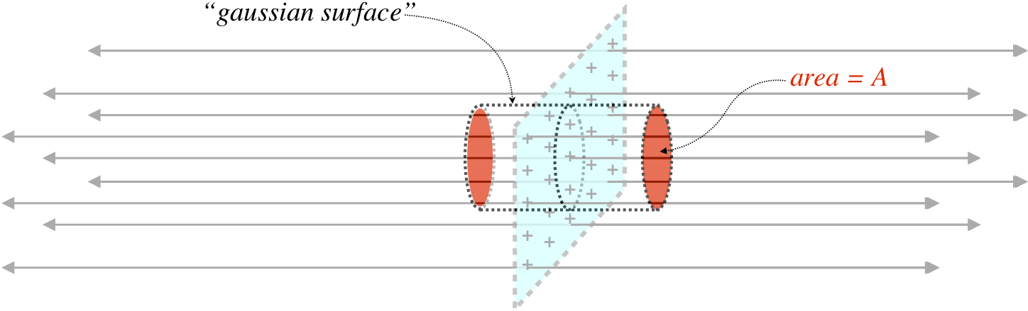
This is a problem we have already solved (Equation 1.3.22). We did it by computing the field of a disk of charge on the axis, then taking the limit as the radius of the disk goes to infinity. That was a lot of math! Let's see how we can do it with Gauss's law. It's clear that an infinite plane of positive charge must create a field that points away from, and perpendicular to, the plane in both directions. Let's choose as our gaussian surface a cylinder whose axis is perpendicular to the plane of charge, with a cross-sectional area \(A\).

Figure 1.7.1 – Gaussian Surface for a Plane of Charge

Alert

One of the hardest ideas to grasp for students learning for the first time about how to use Gauss's law seems to be the idea that the gaussian surface is something we construct ourselves as a problem-solving tool. There is no actual surface present, nor is there a specific unique surface that must be used. To make the solution as simple as possible, the surface should have the two properties given above, and the trick to these problems is conceiving of a surface that does this.

We note that the electric field only passes through the ends of the cylinder, which means that there is no flux through the sides. Also, the field that passes through the ends is parallel to the area vector, so \(\cos\theta=1\) everywhere on that surface. The electric field strength is the same value everywhere on the surface, so it can be pulled out of the integral, which then gives simply the area of the end of the cylinder. The flux is out (positive) at both ends and equal, so they provide equal contributions to the total flux. The total flux out of the cylinder then is simply:

\[ \Phi_E = \cancelto{0}{\Phi_E\left(sides\right)} + \Phi_E\left(left\;end\right) + \Phi_E\left(right\;end\right) \;\;\; \Rightarrow \;\;\;\Phi_E =2EA\]

Now we apply Gauss's law. The amount of charge enclosed in this cylinder is the surface density of the charge multiplied by the area cut out of the plane by the cylinder (like a cookie-cutter), which is clearly equal to \(A\), the area of the ends of the cylinder. Applying Gauss's law gives:

\[ \Phi_E = \dfrac{Q_{encl}}{\epsilon_o} \;\;\; \Rightarrow \;\;\; 2EA = \dfrac{\sigma A}{\epsilon_o} \;\;\; \Rightarrow \;\;\; E = \dfrac{\sigma}{2\epsilon_o}\]

This is exactly the answer we got before! Notice that the final answer comes out to be independent of the length of the cylinder, which means that the field is uniform, and it comes out to be independent of the area of the cylinder as well.

One might well ask, "What if the cylinder didn't have straight sides? That is, what if it bulged in the middle, causing it to enclose more charge? Won't this give a different answer?" The answer is that if the sides of the cylinder aren't straight, then the electric field will pierce the gaussian surface through the sides as well as the ends. The flux through the ends would be the same as before, and the additional flux through the sides would account for the additional enclosed charge.

Field Outside an Infinite Charged Conducting Plane

We have already solved this problem as well (Equation 1.5.6). Solving it with Gauss's law is almost identical to the case above, with one exception: We don't know what the field looks like on both sides of the conductor – we only know that one side of it is charged. But that's fine, because this time we choose our gaussian cylinder so that one end surface is outside the conductor, and the other is inside the metal.

Figure 1.7.2 – Gaussian Surface for a Conducting Plane of Charge

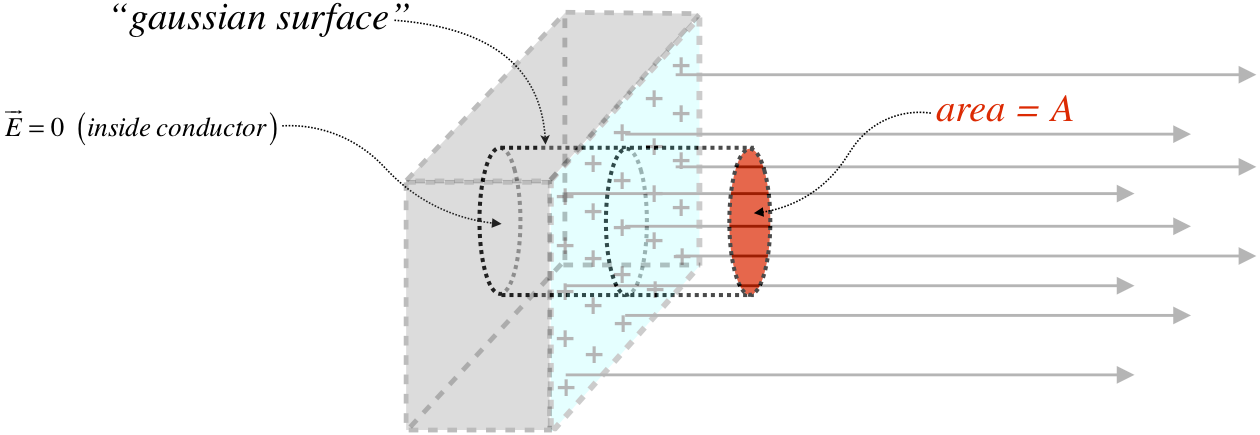
The computation follows exactly as before, with one exception: We know that conductors have zero electric field inside the metal (we are assuming electrostatics here), so there is no electric field flux through that end of the cylinder. The enclosed charge is the same as before, so we get:

\[ \Phi_E = \dfrac{Q_{encl}}{\epsilon_o} \;\;\; \Rightarrow \;\;\; EA = \dfrac{\sigma A}{\epsilon_o} \;\;\; \Rightarrow \;\;\; E = \dfrac{\sigma}{\epsilon_o}\]

Once again, the same answer that we got previously. But there is additional value in this solution that we didn't have before. In our previous approach to this, we made some specific assumptions about the shape of the conducting slab. With Gauss's law, we can even work with a curved surface, for the following reason: When a surface is curved, that curvature is only noticeable when a sufficient amount of that surface is taken into account (e.g. the Earth's surface appears to be flat until you get far enough away from it). In this gauss's law approach, we can make the cross-sectional area of the cylinder as arbitrarily small as we like, and the answer doesn't change. As soon as we make the cross-sectional area "small enough" that the curved conducting surface is effectively flat (i.e. the electric field is constant over the entire end surface of the cylinder), then the answer obtained applies. This means that this answer applies at every conducting surface, if the density is evaluated at a specific position on the surface. In other words, if the charge density on the surface of a conductor at position \(x\) is \(\sigma\left(x\right)\), then the electric field magnitude at that same position in space is:

\[E\left(x\right)=\dfrac{\sigma\left(x\right)}{\epsilon_o}\]

An as we already found, the field is perpendicular to the conducting surface at that point).

Field of an Infinite Line of Charge

Yet another problem we have already solved! As we will see, this one is different from the previous two, in that the field will end up depending upon the dimensions of our gaussian surface. This gives us a field that is not uniform (which it isn't!). Once again, the trick is to define a gaussian surface where the field lines pass through parts of it at right angles, and other parts not at all. The obvious choice is therefore a cylinder.

Figure 1.7.3 – Gaussian Surface for an Infinite Line of Charge

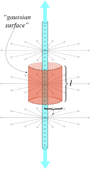
We know from symmetry arguments we have already made in the past that the field points radially outward from the line, which means that the field lines don't pass through the ends of the cylinder, contributing nothing to the total flux. Though the curved surface of the cylinder, the electric field is perpendicular everywhere, and since the cylinder is centered at the line of charge, the field strength is the same everywhere. The total flux is therefore the electric field strength at the cylinder wall multiplied by its area:

\[ \Phi_E = \cancelto{0}{\Phi_E\left(top\right)} + \cancelto{0}{\Phi_E\left(bottom\right)} + \Phi_E\left(sides\right) \;\;\; \Rightarrow \;\;\;\Phi_E =EA=2\pi rlE\]

The enclosed charge is the charge contained between the two ends of the cylinder, which is the linear charge density multiplied by the length of the segment, which is the length of the cylinder. Applying Gauss's law therefore gives:

\[ \Phi_E = \dfrac{Q_{encl}}{\epsilon_o} \;\;\; \Rightarrow \;\;\; 2\pi rlE = \dfrac{\lambda \;l}{\epsilon_o} \;\;\; \Rightarrow \;\;\; E = \dfrac{\lambda}{2\pi\epsilon_o\;r}\]

Again this is in agreement with the answer previously obtained (Equation 1.3.21).

Fields Within Charge Distributions

The reader should not get the impression that electric fields only exist outside of charge distributions, though so far every example has been of this variety. Indeed Gauss's law is very useful for finding fields within charge distributions, and the process is really no different from what is outlined above.

Consider the case of a sphere of charge with a uniform density \(\rho\) and a radius \(R\). We can use Gauss's law to compute the electric field at points within the region of the charge distribution (\(r<R\)), as well as outside the sphere (\(r>R\)). The latter calculation is as simple as those above – the field has spherical symmetry (is radially outward), so we choose a spherical gaussian surface (through which the field will pass orthogonally, and on which the field strength is constant), giving:

\[EA_{sphere}=\dfrac{Q_{encl}}{\epsilon_o} \;\;\; \Rightarrow \;\;\; E\left(r\right) = \dfrac{Q_{encl}}{4\pi\epsilon_or^2} \]

Yes, the field looks exactly like that of a point charge! This will be true for the empty space outside of all spherically symmetric charge distributions, even if the charge density varies with respect to \(r\). As we are not given the value of \(Q\), we are not yet finished with this problem. The density is constant, so the total charge is just the density multiplied by the volume of the charge. Note that this is not the volume of our gaussian surface, which resides outside the sphere, so:

\[E\left(r\right) = \dfrac{\rho V}{4\pi\epsilon_or^2} = \dfrac{\rho \frac{4}{3}\pi R^3}{4\pi\epsilon_or^2} = \dfrac{\rho R^3}{3\epsilon_or^2} \]

Okay, so what about within the charge distribution? The solution is performed in precisely the same way, except that now the spherical gaussian surface has a radius \(r\) that is less than \(R\). So how does this change the answer? Well, there is less charge enclosed than in the previous case. Specifically, this time the entire gaussian surface is filled with charge. Plugging in this new, smaller volume gives:

\[E\left(r\right) = \dfrac{\rho V}{4\pi\epsilon_or^2} = \dfrac{\rho \frac{4}{3}\pi r^3}{4\pi\epsilon_or^2} = \dfrac{\rho}{3\epsilon_o}r \]

Rather than getting weaker with an inverse-square dependence as it gets farther from the center, this field actually gets stronger linearly. This happens until \(r\) reaches the outer surface of the sphere of charge, then after that it follows the point-charge-like inverse-square weakening behavior.

Alert

Whenever one solves a problem that includes multiple regions like this one (one region being inside the charge, and the other outside the charge), it is a good idea to check to make sure that the field is continuous at the boundary. Indeed, in this case, if we plug \(r=R\) into both the interior and exterior solutions, we get the same result. We will see that this is also sometimes used as a condition that we impose to help us solve the problem.

Let's take a moment here to demonstrate how problems where we are looking for fields within charge distributions can also be solved using the local form of Gauss's law. Using this method to solve for fields in empty space is fraught with mathematical nuance that we will avoid, but for regions containing charge it is quite workable, and perhaps even preferable in some cases.

Returning to the uniform sphere of charge, the spherical symmetry suggests that we write the divergence of the spherically-symmetric field in spherical coordinates. For vector fields that are only functions of \(r\) we have:

\[\overrightarrow \nabla \cdot \overrightarrow E\left(r\right) = \dfrac{1}{r^2}\dfrac{d}{dr}\left[r^2 E\left(r\right)\right] \]

We now apply Gauss's law and integrate. Note that this is an indefinite integral, which requires the introduction of an unknown constant of integration. To solve for this constant, we will need to know the boundary condition for the charge distribution. This is a universal feature of this method.

\[ \dfrac{1}{r^2}\dfrac{d}{dr}\left[r^2 E\right] = \dfrac{\rho}{\epsilon_o} \;\;\; \Rightarrow \;\;\; r^2 E = \dfrac{\rho}{\epsilon_o} \int r^2dr = \dfrac{\rho r^3}{3\epsilon_o}+\beta \;\;\; \Rightarrow \;\;\; E\left(r\right) = \dfrac{\rho}{3\epsilon_o}r+\dfrac{\beta}{r^2}\]

Using the solution for outside the charge that we found above, and plugging in \(r=R\) (the boundary), we find that our constant of integration comes out to be zero in this case. Note that we end up with the same field that we found using the integral version.

One thing to note about these two methods is that when the density is not constant, an integral has to be performed either way. Either the charge density appears in the integration of the divergence, or it appears in an integral to compute the charge enclosed within the volume enclosing (note that in this particular case of constant density we only had to multiply the density by the volume, but we will not always be so lucky).

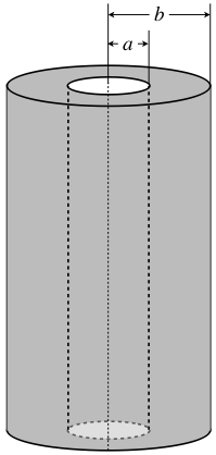
Example \(\PageIndex{1}\)

A very long insulating cylinder is hollow with an inner radius of \(a\) and an outer radius of \(b\). Within the insulating material the volume charge density is given by: \(\rho(R) = \alpha/R\), where \(\alpha\) is a positive constant and \(R\) is the distance from the axis of the cylinder. Choose appropriate gaussian surfaces and use Gauss’s law to find the electric field (magnitude and direction) everywhere.

Solution

There are three distinct regions: (\(0<r<a\)), (\(a<r<b\)), and (\(b<r<\infty\)). For all of these regions, the radial symmetry of the charge distribution ensures that wherever there is electric field, it must point radially outward or inward, and its magnitude must be the same at every point at any fixed radius. A gaussian surface in the shape of a cylinder of radius \(r\) centered within the empty center region would therefore result in a flux of EA, where A is the area of the curved part of this surface, since the electric field is parallel to the area vector everywhere and constant in magnitude. We take each region in turn:

*** \(0<r<a\) ***

The enclosed charge is zero, and since the area isn’t zero, the electric field must be zero for every \(r\) in that empty region.

*** \(a<r<b\) ***

The gaussian surface has a radius \(r\) and a length \(l\). The total electric flux is therefore:

\[\Phi_E=EA=2\pi rlE \nonumber\]

To apply Gauss's law, we need the total charge enclosed by the surface. We have the density function, so we need to integrate it over the volume within the gaussian surface to get the charge enclosed. We use a volume in cylindrical coordinates (\(dV=RdR\;d\theta\;dz\)), and the limits of integration are: \(R:a\rightarrow r\), \(\theta:0\rightarrow 2\pi\), \(z:0\rightarrow l\):

\[Q_{encl} = \int \rho dV = \int\limits_0^l dz \int\limits_0^{2\pi} d\theta \int\limits_a^r \dfrac{\alpha}{R} RdR = 2\pi \alpha l \left(r-a\right) \nonumber \]

Applying Gauss's law gives:

\[ E\left(r\right) = \dfrac{Q_{encl}}{\epsilon_o A} = \dfrac{2\pi \alpha l \left(r-a\right)}{\epsilon_o 2\pi r l} = \boxed{\dfrac{\alpha}{\epsilon_o}\left(1-\dfrac{a}{r}\right)} \nonumber \]

*** \(b<r<\infty\) ***

With the gaussian surface now outside the entire charge distribution, the enclosed charge distribution is all of the charge. We can re-use the work above by simply changing the upper limit in the integral for enclosed charge from \(r\) to \(b\). This gives:

\[Q_{encl} = 2\pi \alpha l \left(b-a\right) \;\;\; \Rightarrow \;\;\; E\left(r\right) = \boxed{\dfrac{\alpha}{\epsilon_o}\left(\dfrac{b-a}{r}\right)}\nonumber \]

Example \(\PageIndex{2}\)

Repeat the previous example for the outer two regions using the local form of Gauss's law. You can assume that you have already determined that \(E=0\) in the hollow cavity, and use this as a boundary condition.

Solution

In cylindrical coordinates, the divergence of a vector field that is only a function of the distance from the \(z\)-axis is given by:

\[\overrightarrow \nabla \cdot \overrightarrow E\left(r\right) = \dfrac{1}{r}\dfrac{d}{dr}\left[rE\left(r\right)\right] \nonumber\]

Now for each of the two regions we apply Gauss's law:

*** \(a<r<b\) ***

We are given the function of the charge density in this region, so plugging that into the divergence formula gives:

\[\overrightarrow \nabla \cdot \overrightarrow E\left(r\right) = \dfrac{\rho}{\epsilon_o} \;\;\; \Rightarrow \;\;\; \dfrac{1}{r}\dfrac{d}{dr}\left[rE\left(r\right)\right] = \dfrac{\alpha}{\epsilon_o r} \;\;\; \Rightarrow \;\;\; \dfrac{d}{dr}\left[rE\left(r\right)\right] = \dfrac{\alpha}{\epsilon_o}\nonumber\]

Now perform the indefinite integral (don't forget the constant of integration! – I will call it \(\beta\)):

\[rE\left(r\right) = \int \dfrac{\alpha}{\epsilon_o}dr = \dfrac{\alpha}{\epsilon_o}r + \beta \;\;\; \Rightarrow \;\;\; E\left(r\right) = \dfrac{\alpha}{\epsilon_o}+\dfrac{\beta}{r} \nonumber\]

The boundary condition at \(r=a\) requires that the electric field is continuous there, which means that it must equal zero there. This allows us to solve for the constant of integration:

\[E\left(a\right) = 0 = \dfrac{\alpha}{\epsilon_o}+\dfrac{\beta}{a} \;\;\; \Rightarrow \;\;\; \beta = -\dfrac{\alpha a}{\epsilon_o} \nonumber \]

Plugging this back in gives us the electric field in the region of the insulator, which agrees with the answer from the previous example:

\[E\left(r\right) = \dfrac{\alpha}{\epsilon_o}\left(1-\dfrac{a}{r}\right) \nonumber\]

*** \(b<r<\infty\) ***

There is no charge in this region, so the charge density is zero. Plugging this into the divergence formula gives:

\[\overrightarrow \nabla \cdot \overrightarrow E\left(r\right) = 0 \;\;\; \Rightarrow \;\;\; \dfrac{d}{dr}\left[rE\left(r\right)\right] = 0 \;\;\; \Rightarrow \;\;\; rE\left(r\right)=constant =\beta \;\;\; \Rightarrow \;\;\; E\left(r\right) = \dfrac{\beta}{r} \nonumber\]

Once again we need to apply a boundary condition to determine \(\beta\). In this case, we match the solution outside the cylinder to that inside the insulator region at \(r=b\):

\[E\left(b\right)=\dfrac{\alpha}{\epsilon_o}\left(1-\dfrac{a}{b}\right) = \dfrac{\beta}{b} \;\;\; \Rightarrow \;\;\; \beta = \dfrac{\alpha}{\epsilon_o}\left(b-a\right) \;\;\; \Rightarrow \;\;\; E\left(r\right) = \dfrac{\alpha}{\epsilon_o}\left(\dfrac{b-a}{r}\right)\nonumber\]

This again agrees with the answer obtained above.

Hollow Conducting Shells

Another common type of problem one can solve with Gauss's law involves no symmetry. A hollow conducting shell (of any shape) has an interesting property: Since the electric field within the metal of such a shell must vanish, then constructing a gaussian surface within the metal, we can see that there must be zero net flux through that surface. This means that the charge enclosed by that shell must be zero. But what if an electric charge is placed in the hollow space? How can Gauss's law then be satisfied? The only way is for charge in the conductor to migrate. If there is a positive charge in the hollow space, then an equal amount negative charge moves to the inside surface of the conducing shell, bringing the total charge within the gaussian surface to zero. If the shell was originally neutrally-charged, then the positive charge abandoned by the migrating negative charge resides on the outer surface of the shell.

Example \(\PageIndex{3}\)

A closed, hollow conductor contains a smaller, closed hollow conductor and a point charge of \(+1Q\) (see the diagram). Free charge trapped within the interior space of the smaller conductor is unknown, but the smaller conductor itself carries a net charge of \(-3Q\), and the larger conductor carries a net charge of \(+5Q\). If a charge of \(-2Q\) is found on the outside surface of the larger conductor, find how much charge resides on the inside surface of the smaller conductor. Assume all the charges on the conductors are at rest at equilibrium.

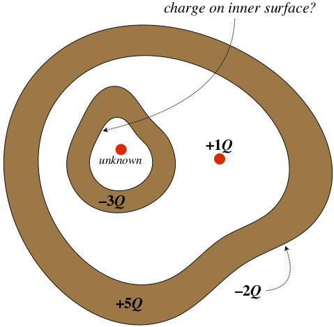
Solution

The total charge on the outer conductor must reside on its surfaces, so if \(-2Q\) is on the outer surface, then there must be \(+7Q\) on its inner surface. Now construct a gaussian surface within the metal of the outer conductor. The zero electric field within the conductor (the charges are static) results in zero flux out of this gaussian surface, which means that there must be no net charge enclosed. The enclosed charge comes in many pieces, and is the sum of the charge on the inner surface of the outside conductor (\(+7Q\)), the free charge outside the smaller conductor (\(+1Q\)), the total charge on the smaller conductor (\(-3Q\)), and the unknown free charge within the smaller conductor. For all of these to add up to zero, the unknown charge must be \(-5Q\). There is also no flux through the inner conductor, so the charge enclosed within gaussian surface constructed within its metal must also be zero. Now that we know the previously-unknown charge is \(-5Q\), there must be a charge of \(+5Q\) on the inner surface of the smaller conductor.