
4.3: Magnetic Field
- Page ID
- 21530

\( \newcommand{\vecs}[1]{\overset { \scriptstyle \rightharpoonup} {\mathbf{#1}} } \)
\( \newcommand{\vecd}[1]{\overset{-\!-\!\rightharpoonup}{\vphantom{a}\smash {#1}}} \)
\( \newcommand{\dsum}{\displaystyle\sum\limits} \)
\( \newcommand{\dint}{\displaystyle\int\limits} \)
\( \newcommand{\dlim}{\displaystyle\lim\limits} \)
\( \newcommand{\id}{\mathrm{id}}\) \( \newcommand{\Span}{\mathrm{span}}\)
( \newcommand{\kernel}{\mathrm{null}\,}\) \( \newcommand{\range}{\mathrm{range}\,}\)
\( \newcommand{\RealPart}{\mathrm{Re}}\) \( \newcommand{\ImaginaryPart}{\mathrm{Im}}\)
\( \newcommand{\Argument}{\mathrm{Arg}}\) \( \newcommand{\norm}[1]{\| #1 \|}\)
\( \newcommand{\inner}[2]{\langle #1, #2 \rangle}\)
\( \newcommand{\Span}{\mathrm{span}}\)
\( \newcommand{\id}{\mathrm{id}}\)
\( \newcommand{\Span}{\mathrm{span}}\)
\( \newcommand{\kernel}{\mathrm{null}\,}\)
\( \newcommand{\range}{\mathrm{range}\,}\)
\( \newcommand{\RealPart}{\mathrm{Re}}\)
\( \newcommand{\ImaginaryPart}{\mathrm{Im}}\)
\( \newcommand{\Argument}{\mathrm{Arg}}\)
\( \newcommand{\norm}[1]{\| #1 \|}\)
\( \newcommand{\inner}[2]{\langle #1, #2 \rangle}\)
\( \newcommand{\Span}{\mathrm{span}}\) \( \newcommand{\AA}{\unicode[.8,0]{x212B}}\)
\( \newcommand{\vectorA}[1]{\vec{#1}} % arrow\)
\( \newcommand{\vectorAt}[1]{\vec{\text{#1}}} % arrow\)
\( \newcommand{\vectorB}[1]{\overset { \scriptstyle \rightharpoonup} {\mathbf{#1}} } \)
\( \newcommand{\vectorC}[1]{\textbf{#1}} \)
\( \newcommand{\vectorD}[1]{\overrightarrow{#1}} \)
\( \newcommand{\vectorDt}[1]{\overrightarrow{\text{#1}}} \)
\( \newcommand{\vectE}[1]{\overset{-\!-\!\rightharpoonup}{\vphantom{a}\smash{\mathbf {#1}}}} \)
\( \newcommand{\vecs}[1]{\overset { \scriptstyle \rightharpoonup} {\mathbf{#1}} } \)
\(\newcommand{\longvect}{\overrightarrow}\)
\( \newcommand{\vecd}[1]{\overset{-\!-\!\rightharpoonup}{\vphantom{a}\smash {#1}}} \)
\(\newcommand{\avec}{\mathbf a}\) \(\newcommand{\bvec}{\mathbf b}\) \(\newcommand{\cvec}{\mathbf c}\) \(\newcommand{\dvec}{\mathbf d}\) \(\newcommand{\dtil}{\widetilde{\mathbf d}}\) \(\newcommand{\evec}{\mathbf e}\) \(\newcommand{\fvec}{\mathbf f}\) \(\newcommand{\nvec}{\mathbf n}\) \(\newcommand{\pvec}{\mathbf p}\) \(\newcommand{\qvec}{\mathbf q}\) \(\newcommand{\svec}{\mathbf s}\) \(\newcommand{\tvec}{\mathbf t}\) \(\newcommand{\uvec}{\mathbf u}\) \(\newcommand{\vvec}{\mathbf v}\) \(\newcommand{\wvec}{\mathbf w}\) \(\newcommand{\xvec}{\mathbf x}\) \(\newcommand{\yvec}{\mathbf y}\) \(\newcommand{\zvec}{\mathbf z}\) \(\newcommand{\rvec}{\mathbf r}\) \(\newcommand{\mvec}{\mathbf m}\) \(\newcommand{\zerovec}{\mathbf 0}\) \(\newcommand{\onevec}{\mathbf 1}\) \(\newcommand{\real}{\mathbb R}\) \(\newcommand{\twovec}[2]{\left[\begin{array}{r}#1 \\ #2 \end{array}\right]}\) \(\newcommand{\ctwovec}[2]{\left[\begin{array}{c}#1 \\ #2 \end{array}\right]}\) \(\newcommand{\threevec}[3]{\left[\begin{array}{r}#1 \\ #2 \\ #3 \end{array}\right]}\) \(\newcommand{\cthreevec}[3]{\left[\begin{array}{c}#1 \\ #2 \\ #3 \end{array}\right]}\) \(\newcommand{\fourvec}[4]{\left[\begin{array}{r}#1 \\ #2 \\ #3 \\ #4 \end{array}\right]}\) \(\newcommand{\cfourvec}[4]{\left[\begin{array}{c}#1 \\ #2 \\ #3 \\ #4 \end{array}\right]}\) \(\newcommand{\fivevec}[5]{\left[\begin{array}{r}#1 \\ #2 \\ #3 \\ #4 \\ #5 \\ \end{array}\right]}\) \(\newcommand{\cfivevec}[5]{\left[\begin{array}{c}#1 \\ #2 \\ #3 \\ #4 \\ #5 \\ \end{array}\right]}\) \(\newcommand{\mattwo}[4]{\left[\begin{array}{rr}#1 \amp #2 \\ #3 \amp #4 \\ \end{array}\right]}\) \(\newcommand{\laspan}[1]{\text{Span}\{#1\}}\) \(\newcommand{\bcal}{\cal B}\) \(\newcommand{\ccal}{\cal C}\) \(\newcommand{\scal}{\cal S}\) \(\newcommand{\wcal}{\cal W}\) \(\newcommand{\ecal}{\cal E}\) \(\newcommand{\coords}[2]{\left\{#1\right\}_{#2}}\) \(\newcommand{\gray}[1]{\color{gray}{#1}}\) \(\newcommand{\lgray}[1]{\color{lightgray}{#1}}\) \(\newcommand{\rank}{\operatorname{rank}}\) \(\newcommand{\row}{\text{Row}}\) \(\newcommand{\col}{\text{Col}}\) \(\renewcommand{\row}{\text{Row}}\) \(\newcommand{\nul}{\text{Nul}}\) \(\newcommand{\var}{\text{Var}}\) \(\newcommand{\corr}{\text{corr}}\) \(\newcommand{\len}[1]{\left|#1\right|}\) \(\newcommand{\bbar}{\overline{\bvec}}\) \(\newcommand{\bhat}{\widehat{\bvec}}\) \(\newcommand{\bperp}{\bvec^\perp}\) \(\newcommand{\xhat}{\widehat{\xvec}}\) \(\newcommand{\vhat}{\widehat{\vvec}}\) \(\newcommand{\uhat}{\widehat{\uvec}}\) \(\newcommand{\what}{\widehat{\wvec}}\) \(\newcommand{\Sighat}{\widehat{\Sigma}}\) \(\newcommand{\lt}{<}\) \(\newcommand{\gt}{>}\) \(\newcommand{\amp}{&}\) \(\definecolor{fillinmathshade}{gray}{0.9}\)Field of a Magnetic Dipole
So far we have not talked about sources of magnetic fields, but even in our discussion of magnetic forces, we have not made any mention of magnetic charges that behave in magnetic fields the same way that electric charges behave in electric fields – with forces that act along the field lines, rather than perpendicular to them. We don't have the equivalent of Coulomb's law for two magnetic point charges, for example. Let's explore this possibility here...
Everyone has at least a passing experience with magnets – little metal disks we stick to refrigerators to hold papers we need to remember. From our experience, we know that if we put two magnets together a certain way, they stick together, and if we turn one of them around, they repel. So they clearly have a directionality to them. The closest analogy in electricity is a dipole. Indeed, if we put two dipoles end-to-end one way, they will attract, and if we turn one of them around, they will repel.
Figure 4.3.1a – Attraction of Aligned Electric Dipoles
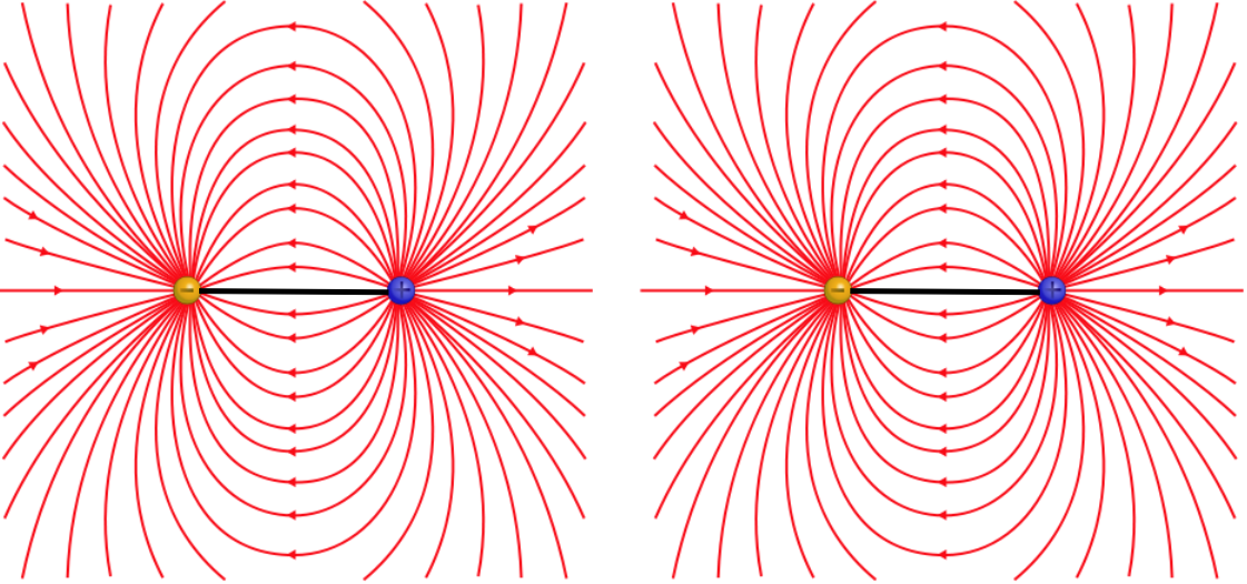
Figure 4.3.1b – Repulsion of Anti-Aligned Electric Dipoles
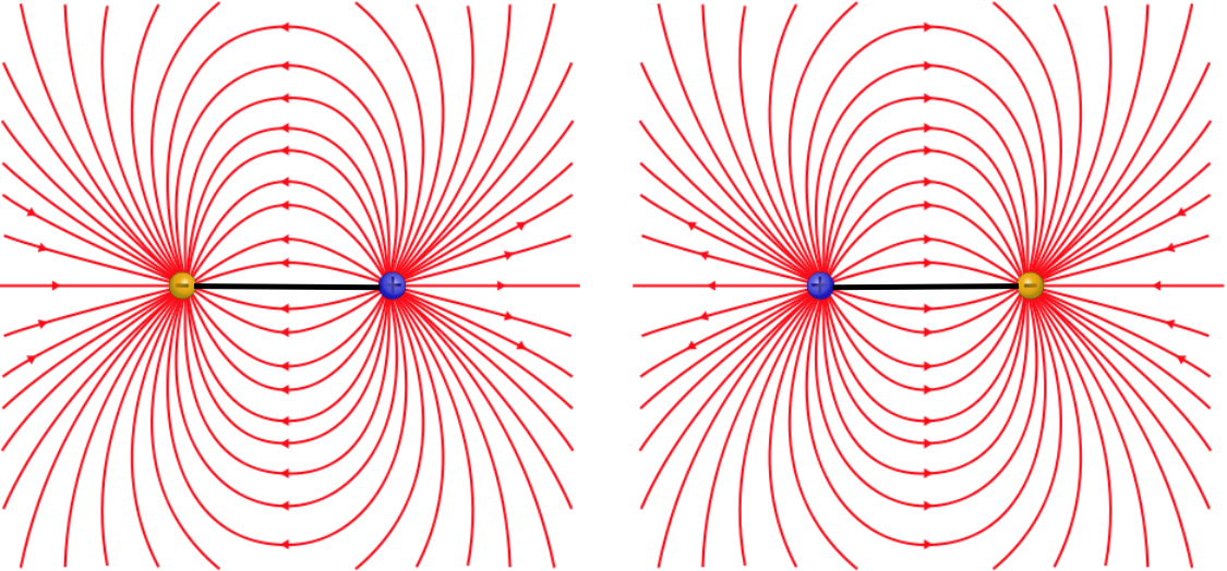
The attraction and repulsion occur because the there is a field created by one dipole that points in the direction outward from the positive charge, and the field gets weaker with distance, so the other dipole will feel a net force according to whichever of the two charges is closer to the dipole creating the field. In magnetism, we call the end of the magnet from which emerges the outward-going field lines the north pole, and the end into which the field lines converge the south pole. From the figures above, it's clear that the dipoles whenever like poles are brought together, and attract when opposite poles are brought together.
Okay, so this looks like a reasonable explanation for how magnets work, so if we want to isolate the two individual magnetic charges (a "north charge" and a "south charge"), all we have to do is cut the magnet in half, right?
Figure 4.3.2a – Isolating Magnetic Charges from a Magnet – An Attempt
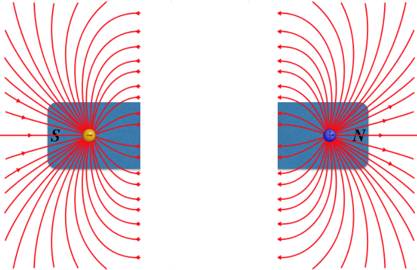
Well, try as we might, this never happens. Instead, every time we cut a magnet with two poles into two pieces, we just get two more magnets with two poles!
Figure 4.3.2b – Isolating Magnetic Charges from a Magnet – What Actually Happens
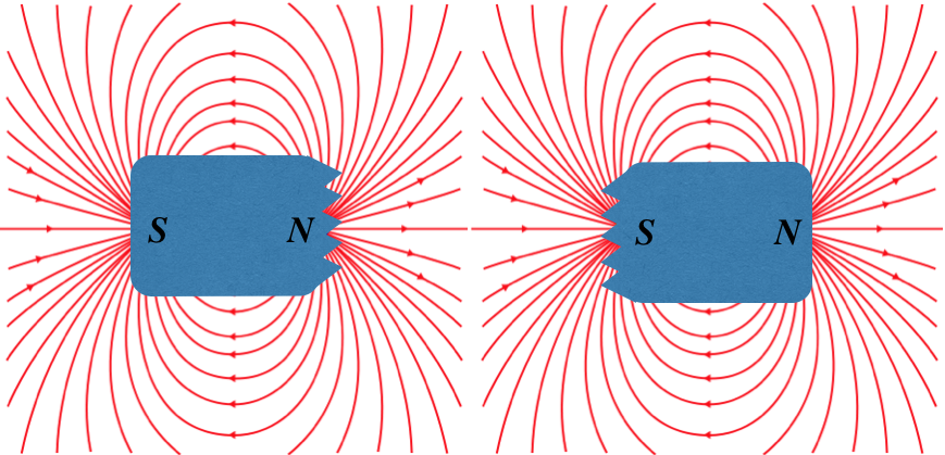
If we examine the the field lines for a bar magnet closely and compare them to an electric dipole field, we see how fundamentally-different the two fields are. For the electric dipole, the field changes direction between the two poles, while for the magnetic case, the field lines continue straight through:
Figure 4.3.3 – Comparing Field Lines of Electric and Magnetic Dipoles
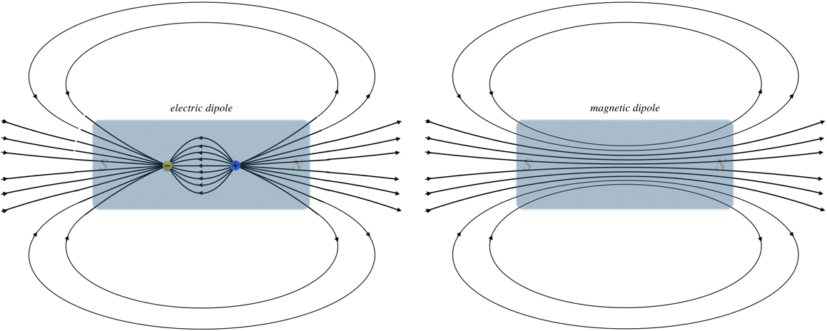
Outside the dipoles, the fields look the same, but they are clearly different, which we can characterize in the following way:
Magnetic field lines always form closed loops, while electric field lines begin and end on electric charges.
Put another way, unlike electric fields which form their dipole fields from two monopoles, there don't seem to be any magnetic monopoles. Or at least we have never been able to detect a magnetic monopole, despite many decades of experimental search for them. It turns out that electromagnetic theory doesn't exclude the possibility of the existence of these point charges of magnetism, but ultimately our theories have to agree with what we observe in experiments, so at least for the moment (and for the duration of this class), we will maintain the position that they simply don't exist.
Gauss's Law for Magnetism
The revelation that our theory of magnetism doesn't include individual magnetic charges has an immediate consequence for the magnetic equivalent of Gauss's law. With magnetic field lines always forming closed loops, any field line that penetrates a Gaussian surface going in one direction (say going into the volume bounded by the surface) must later emerge from that closed surface later in order to form the closed loop. If there is a field line exiting a surface for every field line that enters it, then the net flux must necessarily always be zero. Of course, from Gauss's law, this means that there can never be any charge enclosed, and this makes sense, given that there is no magnetic charge!
Mathematically, we express this Gauss's law for magnetism in either integral or local form:
\[\oint \overrightarrow B\cdot d\overrightarrow A = 0\;,\;\;\;\;\; \overrightarrow \nabla \cdot \overrightarrow B = 0\]
Field of a Moving Point Charge
When we first started discussing magnetism, we noted a force between two current-carrying wires. From there, we focused on the fact that a magnetic field affects only moving electric charges, but it should be equally clear that the source of a magnetic field must also be moving electric charges. One might object that we just said that magnetic fields don't have point sources, so what difference does it make that we insist that the point source be moving? We will see that this makes all the difference, because this leads to a field that doesn't point directly toward or away from that charge – the direction of the field is determined by the direction of the velocity vector.
As different as the magnetic field is from the electric field, there are still so many striking similarities that it is useful to describe the features of the magnetic field from a moving point charge in parallel with the Coulomb electric field. This magnetic analog of the Coulomb field is called the law of Biot & Savart.
- In the Coulomb case, we started with the fact that the field strength is proportional to the magnitude of the charge emitting the field. In the magnetic case, the field strength is also proportional to the magnitude of the charge, but since the charge must also be moving, it turns out that the field strength is also proportional to the charge's speed. This agrees with the observation that there is no magnetic field if the charge is stationary.
- Next we consider how the strength of the field weakens with distance from the source. In this case, the two fields behave identically – with an inverse-square law.
- The direction is where these two fields differ the most. In the Coulomb case, the field points directly toward or away from the point charge. Put another way, if the source charge is at the origin, then the electric field at a position in space described by a position vector \(\overrightarrow r\) points in a direction that is parallel to that position vector. The magnetic field, by contrast points perpendicular to that position vector. This doesn't narrow down the direction, however, as there is an entire plane that is perpendicular to this vector. This is where the velocity vector direction comes in – the magnetic field is also perpendicular to the direction defined by the velocity vector. We already know a way of expressing a vector that is perpendicular to two other vectors at the same time – it must be parallel to the cross product of those two vectors.
Putting all these features together, and including physical constants to make the units work out correctly, we get the following summary:
\[\begin{array}{c} \text{feature} && \text{Coulomb} && \text{Biot-Savart} \\ \text{field source:} && \left|\overrightarrow E\right| \propto q\;\;\text{(charge)} && \left|\overrightarrow B\right| \propto q\left|\overrightarrow v\right|\;\;\text{(moving charge)} \\ \text{field strength with distance:} && \left|\overrightarrow E\right| \propto \dfrac{1}{r^2} && \left|\overrightarrow B\right| \propto \dfrac{1}{r^2} \\ \text{direction:} && \overrightarrow E \parallel \overrightarrow r && \overrightarrow B \parallel \overrightarrow v \times \overrightarrow r \\ \text{physical constant:} && \overrightarrow E = \left(\dfrac{1}{4\pi\epsilon_o}\right) \dfrac{q\overrightarrow r}{r^3} && \overrightarrow B = \left(\dfrac{\mu_o}{4\pi}\right) \dfrac{q\overrightarrow v \times \overrightarrow r}{r^3}\end{array}\]
The physical constant that makes the units work out for the force is called the permeability of free space:
\(\mu_o = 4\pi\times 10^{-7} \frac{T\cdot m}{A}\)
Yes, that is exactly \(4\pi\) in that constant. The unit of Tesla was constructed to come out to Newtons, which explains why the \(4\pi\) cancels-out in Biot-Savart's law. One might wonder why we bother to introduce the constant this way at all, and the answer to this question will become clear later. Right now the short answer is that it will parallel very closely the role that \(\epsilon_o\) plays in electricity.
While it is not obvious from the final form of the equation for the magnetic field, the resulting field is a circle centered at the line passing through the charge along the direction of motion:
Figure 4.3.4 – Magnetic Field of a Moving Point Charge
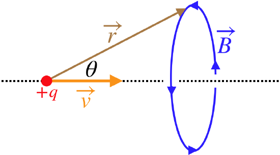
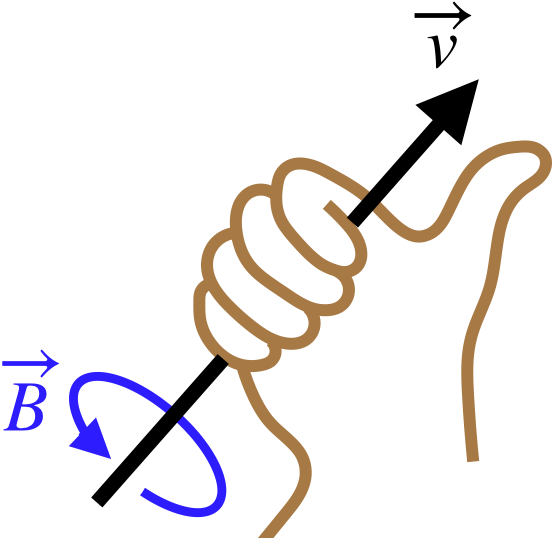
Rather than using the right-hand-rule for the cross-product \(\overrightarrow v \times \overrightarrow r\) (which gives the direction of the magnetic field at a specific point in space), we can get a bigger-picture idea of the magnetic field lines by using a different right-hand-rule: Point the thumb of the right hand in the direction of motion of the charge, and the magnetic field direction everywhere in space forms closed circles around the line of motion in the direction that the fingers curl.
Figure 4.3.5 – Right-Hand-Rule for Magnetic Field
Field of a Current-Carrying Wire
It is far more common to have physical situations where a magnetic field is created by a current-carrying wire than by a point charge. Fortunately, we already know how to convert from moving point charges to current elements:
\[I\;\overrightarrow {dl} \leftrightarrow dq \;\overrightarrow v\]
We therefore get this for a line of current from the law of Biot & Savart:
\[\overrightarrow B = \int d\overrightarrow B = \int\left[\left(\dfrac{\mu_o}{4\pi}\right)\dfrac{I}{r^2}\overrightarrow {dl} \times \widehat r\right] = \dfrac{\mu_o}{4\pi}\int \dfrac{I{\overrightarrow{dl}} \times \overrightarrow r}{r^3} \]
We can now use this result to continue building our "toolbox" of reusable solutions of common physical sources.