4.2: Magnetic Moment and Torque

Torque on a Loop of Wire

Let's use our result for the force on a segment of wire to analyze the case of the effect of a magnetic field on a closed loop of wire. We will choose a simple geometry for this analysis – a rectangular loop of wire with two sides parallel to a uniform magnetic field.

Figure 4.2.1 – Closed Rectangular Loop of Wire in a Uniform Magnetic Field

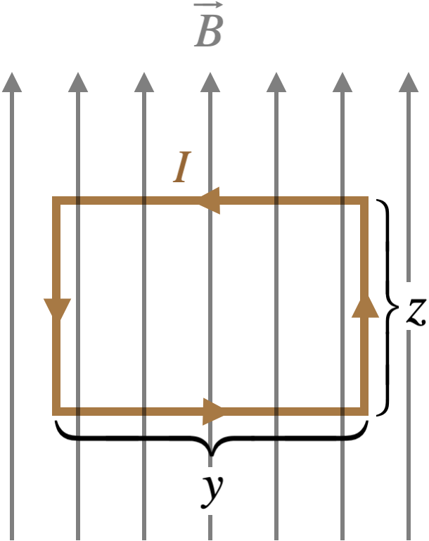
Here are the main features of this set-up:

• The vertical sides of the rectangular loop are parallel to the magnetic field, so the force on every element is zero, adding up to a total of zero force on each of those sides.
• The horizontal sides of the rectangular loop are perpendicular to the field, so the sine of the angle that appears in the cross-product is exactly equal to one.
• The magnetic field is uniform, and the current doesn’t change direction, so combining this with the previous observation, we get a force on each of these segments equal to the same value: \(IyB\).
• We can work out the directions of the forces on these two segments in two ways: Using the right-hand-rule, or plugging-in the unit vectors for the directions of the current and magnetic field, and computing the cross-product. Doing so reveals that the force on the top segment is into the page, while the force on the bottom segment is out of the page.

The forces on the horizontal segments cancel, resulting in zero net force on the loop, but of course there is a net torque. Choosing an axis that is a horizontal line passing through the centers of the two vertical segments, we can compute the net torque on the loop. Choosing the positive torque direction to be to the left, the forces on top and bottom both generate torques in that positive direction, so:

\[\tau_{net} = F_{top}\left(\dfrac{z}{2}\right) + F_{bottom}\left(\dfrac{z}{2}\right) = 2\left(IyB\right)\left(\dfrac{z}{2}\right) = I\left(yz\right)B\]

Magnetic Dipole Moment

Here we introduce a shortcut for future torque calculations. The quantity \(yz\) is the area of the loop, \(A\). In future applications, we may have the current fed into the loop by a single wire, which is wound around th perimeter several times. The force exerted on each side of the loop (and therefore the torque) will then be multiplied by the number of turns in the wire, \(N\). The product of \(N\), \(I\), and \(A\) is written as a single quantity \(\mu\), giving the magnitude of the torque for this case the simple form of \(\tau = \mu B\).

If this loop turns upon its axis, then the moment arm shrinks. For example, if the top of the loop rotates back and the bottom rotates forward by \(90^o\), then the forces on those segments will be directly away from each other. These forces act straight through the axis, so the torque they produce is zero. We know that torque and magnetic field are both vectors, and the torque created is related to the orientation of the loop in the field. We can account for the loop orientation by defining a magnetic dipole moment:

\[\overrightarrow \mu \equiv NI\overrightarrow A\]

The vector \(\overrightarrow A\) has a magnitude equal to the area of the loop, and has a direction that is perpendicular to the plane of the loop, in the direction defined as follows: Curl the fingers of your right hand in a direction that traces the direction of the current around the loop, and the thumb of that hand points the direction of the vector. For example, the loop in Figure 4.2.1 would have a magnetic moment that points out of the page.

The torque vector can now be calculated from the magnetic dipole moment in the same way that the torque exerted on an electric dipole was calculated:

\[\overrightarrow\tau_{electric} = \overrightarrow p \times \overrightarrow E \;\;\;\Leftrightarrow\;\;\; \overrightarrow\tau_{magnetic} = \overrightarrow \mu \times \overrightarrow B\]

We can see that this works for the case shown in Figure 4.2.1: The angle between the magnetic dipole moment (which points out of the page) and the magnetic field is \(90^o\), so the sine of the angle between these vectors that appears in the cross product is 1, giving the answer we found above. When the loop rotates around the horizontal axis, the angle between the magnetic dipole moment and the field changes, reducing the moment arms of the forces by a factor of \(\sin\theta\) – exactly the amount accounted-for in the cross-product. When the loop rotates to the point where its plane is perpendicular to the field, the magnetic moment and field are parallel, making the torque zero, as we found above.

Example \(\PageIndex{1}\)

A \(2.00\;A\) current flows through a circular conductor, which has a radius of \(12.0\;cm\) and lies in the \(x\)-\(y\) plane. When viewed from the +\(z\)-axis, the current is flowing clockwise. This loop is in the presence of a uniform magnetic field given by:

\[\overrightarrow B = B_o\left(\widehat i-3\widehat j + 2\widehat k\right)\;,\;\;\;\;where:\;\;B_o=1.50T\nonumber\]

Find the torque (vector) exerted on the conductor.

Solution

To find the torque vector, we first need the magnetic moment. We calculate that to be (use RHR for direction):

\[\overrightarrow \mu = IA\left(-\widehat k\right) = \left(2.00A\right)\pi\left(0.12m\right)^2\left(-\widehat k\right) = \left(-9.05\times 10^{-2} A\cdot m^2\right)\widehat k\nonumber\]

Now just plug into the formula for torque:

\[\overrightarrow \tau = \overrightarrow \mu \times \overrightarrow B = \left[\left(-9.05\times 10^{-2} A\cdot m^2\right)\widehat k\right]\times\left[\left(1.50T\right)\left(\widehat i-3\widehat j + 2\widehat k\right)\right] = -\left(0.136\;N\cdot m\right)\left(3\widehat i + \widehat j\right)\nonumber\]

Although we derived the formula for the magnetic dipole moment using a rectangle, it turns out that as long as the loop lies in a plane, the formula works no matter what shape it is. As an illustrative example, we will solve the torque on a circular loop. This is a more difficult example than the rectangle, for reasons that will become clear, but it does demonstrate important tools for integrating infinitesimal contributions and dealing with vector products.

Figure 4.2.2a – Torque on a Closed Circular Loop of Wire in a Uniform Magnetic Field

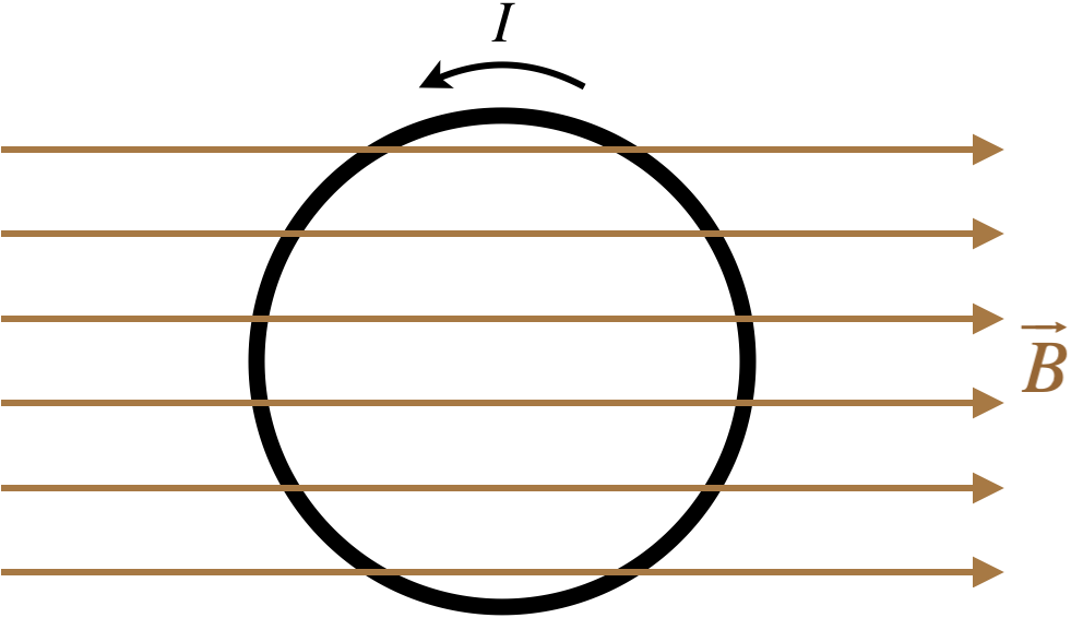
Much like we did for integrating charge distributions to obtain fields, we start by introducing a coordinate system (make sure it is right-handed, i.e. choose the axes so that \(\widehat i \times \widehat j = \widehat k\)), select an infinitesimal piece os the loop, and describe it in terms of the coordinates, labeling whatever variables we will need to know along the way.

Figure 4.2.2b – Torque on a Closed Circular Loop of Wire in a Uniform Magnetic Field

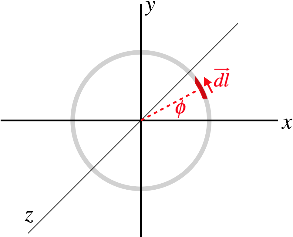
Here we have chosen to place the loop in the \(x\)-\(y\) plane, and the magnetic field points in the \(+x\)-direction. An infinitesimal slice of wire has been selected at an angle \(\phi\) up from the \(+x\)-axis.

Next we need to express the vector \(\overrightarrow {dl}\) mathematically. Its magnitude is the length of an infinitesimal segment of arc, which is \(R\;d\phi\). The direction is trickier to come up with, but blowing up the picture and doing a bit of geometry, we can determine its components:

Figure 4.2.3 – Writing the Current Element Vector

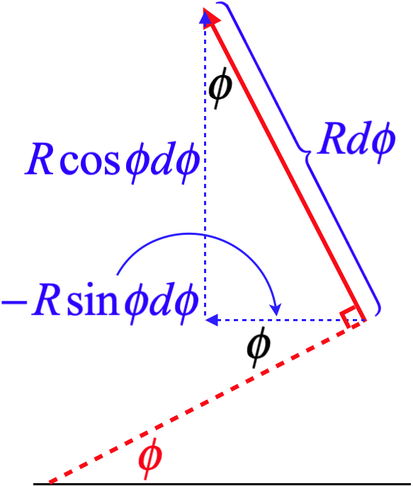
Putting it together into a single vector:

\[\overrightarrow {dl} = R\;d\phi\left(-\sin\phi\;\widehat i + \cos\phi\;\widehat j\right)\]

We now have everything we need. As complicated as the geometry is with the force and then the torque, we don't have to track it – all we need to do is do the vector math properly. For example, the force on the current element is:

\[d\overrightarrow F = I \overrightarrow {dl} \times \overrightarrow B = I\left[R\;d\phi\left(-\sin\phi\;\widehat i + \cos\phi\;\widehat j\right)\right]\times\left[B \;\widehat i\right]\]

Recalling the cross products of unit vectors from Physics 9A, we plug in \(\widehat i\times\widehat i = 0\) and \(\widehat j\times\widehat i = -\widehat k\), and the force on this element becomes:

\[d\overrightarrow F = IRB\cos\phi\;d\phi \left(-\widehat k\right)\]

To get the torque, we choose the origin as a reference point, and compute the infinitesimal contribution to the torque directly. Plugging in the position vector and doing the vector math gives:

\[d\overrightarrow \tau = \overrightarrow r \times d\overrightarrow F = \left(R\cos\phi\;\widehat i + R\sin\phi\;\widehat j\right)\times \left(-IRB\cos\phi\;d\phi\;\widehat k\right) = -IR^2B\;d\phi\left[\cos^2\phi \left(-\widehat j\right) + \sin\phi \cos\phi \left(\widehat i\right)\right]\]

All that remains is to add up all of the torque contributions, which means integrating over the angle \(\phi\) from \(0\rightarrow 2\pi\):

\[\overrightarrow \tau =-IR^2B\int\limits_0^{2\pi}d\phi\left[\cos^2\phi \left(-\widehat j\right) + \sin\phi \cos\phi \left(\widehat i\right)\right] = IR^2B\left[\pi \;\widehat j-0 \;\widehat i\right]=I\left(\pi R^2\right)B\;\widehat j\]

Sure enough, the magnitude of the torque comes out to be \(\mu\;B\), where \(\mu=IA\). And using the right-hand-rule to get the direction of the magnetic moment (out of the page) followed by the direction of the torque from the right-hand-rule applied to \(\overrightarrow\mu\times\overrightarrow B\), confirms that the direction works as well.

This problem seemed very daunting because the direction of \(\overrightarrow {dl}\) is changing everywhere on the circle, but once this vector is written in terms of \(\phi\) and the unit vectors, the math does the rest!

Comparing Magnetic to Electric

We found that we could do more with electric dipoles than just compute torques, and the same is true for magnetic dipoles. The nice thing is that we don't have to work through everything again – the same results simply translate-over by replacing \(\overrightarrow p\) with \(\overrightarrow \mu\), and \(\overrightarrow E\) with \(\overrightarrow B\). So we have the potential energy of a dipole in a field:

\[U_{electric} = -\overrightarrow p \cdot \overrightarrow E \;\;\;\Leftrightarrow\;\;\; U_{magnetic} = -\overrightarrow \mu \cdot \overrightarrow B\]

As we saw with the electric dipole, we can explain the instability of the anti-aligned position in terms of having a maximum potential energy.

Example \(\PageIndex{2}\)

The device shown in the diagram consists of a square loop through which flows a steady current, located in a uniform magnetic field, and attached to an axle that turns a wheel. Around the wheel is wound a (massless) string (the string comes down over the front of the wheel as shown in the diagram), from which hangs a mass. The mass rises and falls such that it is at rest when the plane of the loop is vertical, and is again at rest when the plane of the loop is horizontal (i.e. the loop does not spin all the way around, but rather goes back-and-forth).

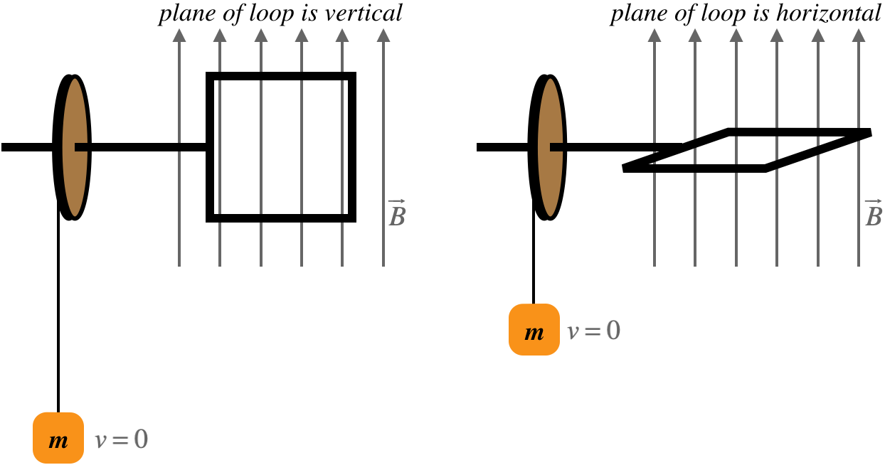
1. In which direction (as seen by our view of the loop being in the vertical plane) is the current going, clockwise or counter-clockwise?
2. Use the values below to determine the amount of current flowing through the loop.

\[g = 9.8\;\frac{m}{s^2} \;,\;\;\; m=0.45\;kg\;,\;\;\; B=1.2\;T\;,\;\;\; \text{length of the sides of the loop} = 0.54m\;,\;\;\; \text{radius of wheel} = 0.25m\nonumber\]

Solution

a. The magnetic field turns the loop such that the top segment goes into the page. Curling our fingers in that direction gives a direction of torque that is to the left. The torque direction comes from the cross product of magnetic moment and field. The field is up, so for the cross product to be to the left, the fingers have to curl from out of the page upward. Therefore the magnetic moment points out of the page. Curling our fingers counterclockwise gives this direction, so that is the direction of the current.

b. The system conserves energy, and the mass is moving at neither the top nor the bottom of its journey, so the kinetic energy doesn’t change. Therefore all of the energy changes are in the form of potential energy. At the top of its journey the mass gains gravitational potential energy, and this must have come from the magnetic potential energy of the dipole in the field. The wheel turns through an angle of \(\frac{\pi}{2}\), so we can figure out how much string is wound up by the wheel (which equals the change in height of the mass). This is then used to find the change in gravitational PE:

\[\Delta y = r\theta = \left(0.25\;m\right)\left(\dfrac{\pi}{2}\right) = 0.39\;m\;\;\;\Rightarrow\;\;\; \Delta U_{grav} = mg\Delta y = \left(0.45\;kg\right)\left(9.8\;\frac{m}{s^2}\right)\left(0.39\;m\right) = 1.7\;J\nonumber\]

Next calculate the potential energy change of the dipole in the field in terms of the current. The magnetic moment starts at an angle of 90º with the field, and ends at an angle of 0º:

\[\Delta U_{mag} = \left(-\mu B \cos 0^o\right) - \left(-\mu B \cos 90^o\right) = -IAB = -I \left(0.54\;m\right)^2\left(1.2\;T\right) = -I\left(0.35\;Tm^2\right)\nonumber\]

Now use energy conservation to solve for the current:

\[0=\Delta U_{grav} +\Delta U_{mag}+\Delta KE = 1.7J -I\left(0.35\;Tm^2\right) + 0 \;\;\;\Rightarrow\;\;\; I = \dfrac{1.7\;J}{0.35\;Tm^2} = 4.9\;A\nonumber\]

It is useful to make the direct comparison of these two dipoles in their respective fields with a diagram.

Figure 4.2.4 – Comparing Electric and Magnetic Dipoles

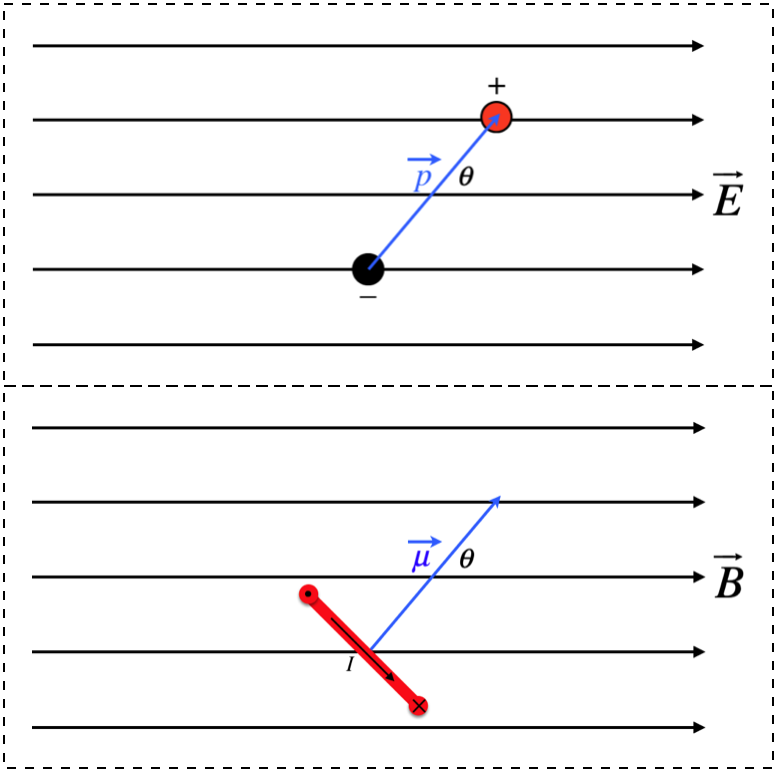
The two physical situations are very different, but viewing it purely in terms of the vectors, they are identical.

There is one last feature of dipoles we need to address – how they react to non-uniform fields. Consider an electric dipole in an electric field that gets stronger along a specific direction. When we discussed torque we used a uniform field, and found that their was no net force on the dipole. But when the field is not uniform, then half of the dipole can be in a region where the field is stronger than the region where the other half of the dipole is, resulting in more force on one part of the dipole than the other, and a net force on the dipole as a whole.

Figure 4.2.5 – Net Force on an Electric Dipole from a Non-Uniform Field

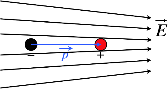
While this is clear for the electric dipole, it's not so obvious for the magnetic dipole, which doesn't have two separated charges.

Figure 4.2.6 – Net Force on an Magnetic Dipole from a Non-Uniform Field

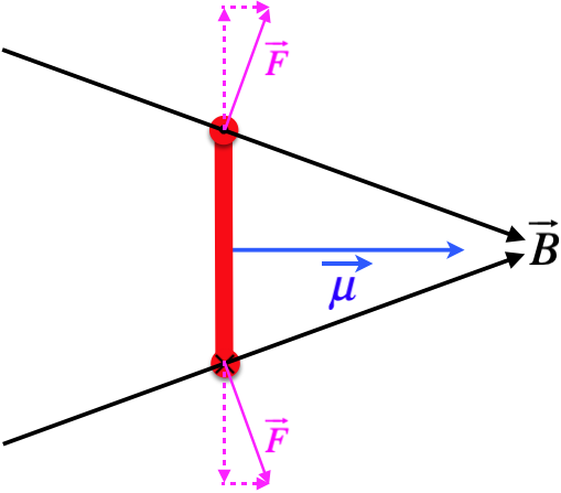
The figure above depicts the side-view of a rectangular loop in a magnetic field that gets stronger to the right (the field lines get closer). The current is circulating clockwise when viewed from the left, so that it is going into the page in the bottom segment of the rectangle, and out of the page in the top segment. The force on the top and bottom segments must be perpendicular to the field, so there are horizontal components of this force that add together, and vertical parts that cancel, the net force being to the right, just as it is in the analogous case for the electric dipole.

We can actually express the amount of net force exerted by the non-uniform field in terms of the rate at which the field changes along the direction of the force, using the fact that the force is the negative gradient of the potential energy. Letting the dipole moment be aligned with the field (a position into which the torque will seek to turn it), we get:

\[\begin{array}{l} \text{electric:} && F_x = -\dfrac{\partial}{\partial x} U_E = -\dfrac{\partial}{\partial x} \left(-\overrightarrow p \cdot \overrightarrow E\right) = -\dfrac{\partial}{\partial x} \left(-p_xE_x\right) = +p_x\dfrac{\partial E_x}{\partial x} \\ \text{magnetic:} && F_x = -\dfrac{\partial}{\partial x} U_B = -\dfrac{\partial}{\partial x} \left(-\overrightarrow \mu \cdot \overrightarrow B\right) = -\dfrac{\partial}{\partial x} \left(-\mu_xB_x\right) = +\mu_x\dfrac{\partial B_x}{\partial x} \end{array}\]

A DC Motor

By creating a torque in a conducting loop that carries a current, we can have it do work. That is, we have the makings of an electric motor. There is one problem to overcome. As the coil turns, the direction of the magnetic moment turns with it. If the magnetic field is unchanging, then the rotation of the magnetic moment will cause the torque to reverse direction, which means the torque cause the loop to accelerate the opposite direction. This makes the coil oscillate back-and-forth, rather than rotate in a single direction. One way to fix this is to provide an emf that switches direction periodically, so that the current flips when the magnetic moment is about to provide the wrong torque. The figure below provides a simple design that fixes this problem with an unchanging emf.

Figure 4.2.7 – A Direct-Current Motor

The steady source of constant magnetic field is a bar magnet (something we will discuss in a future section). The coil rotates, but the motor includes a part called a commutator that has the effect of reversing the direction of the current at just the right moment. This consists of a ring with a break in it that rotates inside two rubbing connections. When the coil has rotated \(90^o\) from the position shown in the diagram, the connection is broken briefly, and a new connection is then created which reverses the current in the wire, but keeps it going the same direction in space. In terms of the figure, when the coil turns past \(90^o\), the current going away from the wheel in the purple segment, rather than toward it, but the current is still goiing toward the wheel in the segment closest to the north magnet, so the direction of the torque remains the same. Put another way, the commutator keeps the magnetic moment of the coil pointing in a direction that always has a component downward – when it is about to start pointing upward, the current direction flips.