
7.3: Energy in Gravitational Systems
- Page ID
- 18420

\( \newcommand{\vecs}[1]{\overset { \scriptstyle \rightharpoonup} {\mathbf{#1}} } \)
\( \newcommand{\vecd}[1]{\overset{-\!-\!\rightharpoonup}{\vphantom{a}\smash {#1}}} \)
\( \newcommand{\id}{\mathrm{id}}\) \( \newcommand{\Span}{\mathrm{span}}\)
( \newcommand{\kernel}{\mathrm{null}\,}\) \( \newcommand{\range}{\mathrm{range}\,}\)
\( \newcommand{\RealPart}{\mathrm{Re}}\) \( \newcommand{\ImaginaryPart}{\mathrm{Im}}\)
\( \newcommand{\Argument}{\mathrm{Arg}}\) \( \newcommand{\norm}[1]{\| #1 \|}\)
\( \newcommand{\inner}[2]{\langle #1, #2 \rangle}\)
\( \newcommand{\Span}{\mathrm{span}}\)
\( \newcommand{\id}{\mathrm{id}}\)
\( \newcommand{\Span}{\mathrm{span}}\)
\( \newcommand{\kernel}{\mathrm{null}\,}\)
\( \newcommand{\range}{\mathrm{range}\,}\)
\( \newcommand{\RealPart}{\mathrm{Re}}\)
\( \newcommand{\ImaginaryPart}{\mathrm{Im}}\)
\( \newcommand{\Argument}{\mathrm{Arg}}\)
\( \newcommand{\norm}[1]{\| #1 \|}\)
\( \newcommand{\inner}[2]{\langle #1, #2 \rangle}\)
\( \newcommand{\Span}{\mathrm{span}}\) \( \newcommand{\AA}{\unicode[.8,0]{x212B}}\)
\( \newcommand{\vectorA}[1]{\vec{#1}} % arrow\)
\( \newcommand{\vectorAt}[1]{\vec{\text{#1}}} % arrow\)
\( \newcommand{\vectorB}[1]{\overset { \scriptstyle \rightharpoonup} {\mathbf{#1}} } \)
\( \newcommand{\vectorC}[1]{\textbf{#1}} \)
\( \newcommand{\vectorD}[1]{\overrightarrow{#1}} \)
\( \newcommand{\vectorDt}[1]{\overrightarrow{\text{#1}}} \)
\( \newcommand{\vectE}[1]{\overset{-\!-\!\rightharpoonup}{\vphantom{a}\smash{\mathbf {#1}}}} \)
\( \newcommand{\vecs}[1]{\overset { \scriptstyle \rightharpoonup} {\mathbf{#1}} } \)
\( \newcommand{\vecd}[1]{\overset{-\!-\!\rightharpoonup}{\vphantom{a}\smash {#1}}} \)
\(\newcommand{\avec}{\mathbf a}\) \(\newcommand{\bvec}{\mathbf b}\) \(\newcommand{\cvec}{\mathbf c}\) \(\newcommand{\dvec}{\mathbf d}\) \(\newcommand{\dtil}{\widetilde{\mathbf d}}\) \(\newcommand{\evec}{\mathbf e}\) \(\newcommand{\fvec}{\mathbf f}\) \(\newcommand{\nvec}{\mathbf n}\) \(\newcommand{\pvec}{\mathbf p}\) \(\newcommand{\qvec}{\mathbf q}\) \(\newcommand{\svec}{\mathbf s}\) \(\newcommand{\tvec}{\mathbf t}\) \(\newcommand{\uvec}{\mathbf u}\) \(\newcommand{\vvec}{\mathbf v}\) \(\newcommand{\wvec}{\mathbf w}\) \(\newcommand{\xvec}{\mathbf x}\) \(\newcommand{\yvec}{\mathbf y}\) \(\newcommand{\zvec}{\mathbf z}\) \(\newcommand{\rvec}{\mathbf r}\) \(\newcommand{\mvec}{\mathbf m}\) \(\newcommand{\zerovec}{\mathbf 0}\) \(\newcommand{\onevec}{\mathbf 1}\) \(\newcommand{\real}{\mathbb R}\) \(\newcommand{\twovec}[2]{\left[\begin{array}{r}#1 \\ #2 \end{array}\right]}\) \(\newcommand{\ctwovec}[2]{\left[\begin{array}{c}#1 \\ #2 \end{array}\right]}\) \(\newcommand{\threevec}[3]{\left[\begin{array}{r}#1 \\ #2 \\ #3 \end{array}\right]}\) \(\newcommand{\cthreevec}[3]{\left[\begin{array}{c}#1 \\ #2 \\ #3 \end{array}\right]}\) \(\newcommand{\fourvec}[4]{\left[\begin{array}{r}#1 \\ #2 \\ #3 \\ #4 \end{array}\right]}\) \(\newcommand{\cfourvec}[4]{\left[\begin{array}{c}#1 \\ #2 \\ #3 \\ #4 \end{array}\right]}\) \(\newcommand{\fivevec}[5]{\left[\begin{array}{r}#1 \\ #2 \\ #3 \\ #4 \\ #5 \\ \end{array}\right]}\) \(\newcommand{\cfivevec}[5]{\left[\begin{array}{c}#1 \\ #2 \\ #3 \\ #4 \\ #5 \\ \end{array}\right]}\) \(\newcommand{\mattwo}[4]{\left[\begin{array}{rr}#1 \amp #2 \\ #3 \amp #4 \\ \end{array}\right]}\) \(\newcommand{\laspan}[1]{\text{Span}\{#1\}}\) \(\newcommand{\bcal}{\cal B}\) \(\newcommand{\ccal}{\cal C}\) \(\newcommand{\scal}{\cal S}\) \(\newcommand{\wcal}{\cal W}\) \(\newcommand{\ecal}{\cal E}\) \(\newcommand{\coords}[2]{\left\{#1\right\}_{#2}}\) \(\newcommand{\gray}[1]{\color{gray}{#1}}\) \(\newcommand{\lgray}[1]{\color{lightgray}{#1}}\) \(\newcommand{\rank}{\operatorname{rank}}\) \(\newcommand{\row}{\text{Row}}\) \(\newcommand{\col}{\text{Col}}\) \(\renewcommand{\row}{\text{Row}}\) \(\newcommand{\nul}{\text{Nul}}\) \(\newcommand{\var}{\text{Var}}\) \(\newcommand{\corr}{\text{corr}}\) \(\newcommand{\len}[1]{\left|#1\right|}\) \(\newcommand{\bbar}{\overline{\bvec}}\) \(\newcommand{\bhat}{\widehat{\bvec}}\) \(\newcommand{\bperp}{\bvec^\perp}\) \(\newcommand{\xhat}{\widehat{\xvec}}\) \(\newcommand{\vhat}{\widehat{\vvec}}\) \(\newcommand{\uhat}{\widehat{\uvec}}\) \(\newcommand{\what}{\widehat{\wvec}}\) \(\newcommand{\Sighat}{\widehat{\Sigma}}\) \(\newcommand{\lt}{<}\) \(\newcommand{\gt}{>}\) \(\newcommand{\amp}{&}\) \(\definecolor{fillinmathshade}{gray}{0.9}\)Gravitational Potential Energy
We showed in Section 3.2 that our terrestrial model of gravity is a conservative force, and it certainly seems reasonable to assume that universal gravitation is as well, but really we should check to see if this is the case. In Section 3.6 we outlined a procedure for determining whether a force is conservative or not – basically it consists of trying to construct a potential energy function whose gradient equals the force, and if we succeed, then the force is conservative. If we can show that it is impossible to do this, then the force is non-conservative. Let's see what happens when we bring this to bear on gravitation.
Let's start by writing the gravity force in cartesian coordinates:
\[ \overrightarrow F \left(x,y,z\right) = -\dfrac{GMm}{r^2} \widehat r = -\dfrac{GMm}{r^3} \overrightarrow r = -\dfrac{GMm}{\left(x^2+y^2+z^2\right)^\frac{3}{2}} \left(x \widehat i + y \widehat j + z \widehat k \right) \]
Consider next the following partial derivative:
\[ \dfrac{\partial}{\partial x} \left(x^2+y^2+z^2\right)^{-\frac{1}{2}} = -\frac{1}{2}\left(x^2+y^2+z^2\right)^{-\frac{3}{2}}\left(2x\right) = \dfrac{-x}{\left(x^2+y^2+z^2\right)^{\frac{3}{2}}} \]
This is precisely the \(x\)-component of the gravitational force. Obviously partial derivatives with respect to \(y\) and \(z\) yield similar results – the \(y\) and \(z\) components of the gravitational force. This means we can immediately define a potential energy function whose negative gradient is the force:
\[ U\left(x,y,z\right) = \dfrac{-GMm}{\left(x^2+y^2+z^2\right)^\frac{1}{2}} + U_o \;\;\; \Rightarrow \;\;\; U\left(r\right) = \dfrac{-GMm}{r} + U_o\]
We could have saved ourselves a lot of trouble if we happened to know a useful fact from vector calculus: The gradient of a function that is purely a function of \(r\) can be written as:
\[ \overrightarrow \nabla U\left(r\right) = \dfrac{d}{dr} U\left(r\right) \widehat r \]
So:
\[ \overrightarrow F = -\overrightarrow \nabla U\left(r\right) = -\dfrac{d}{dr}\left[\dfrac{-GMm}{r}+U_o\right] \widehat r = -\dfrac{GMm}{r^2} \widehat r \]
As with other potential energy functions for another physical system that we have discussed (the intermolecular forces described by the Lennard-Jones potential), we typically choose our arbitrary constant of integration such that the potential energy falls off to zero at infinity. In the case of our gravitational potential energy, this gives what we will use for the potential energy function henceforth:
\[ U_{grav}\left(r\right) = \dfrac{-GMm}{r} \]
A graph of this function looks like this:
Figure 7.3.1 – Gravitational Potential
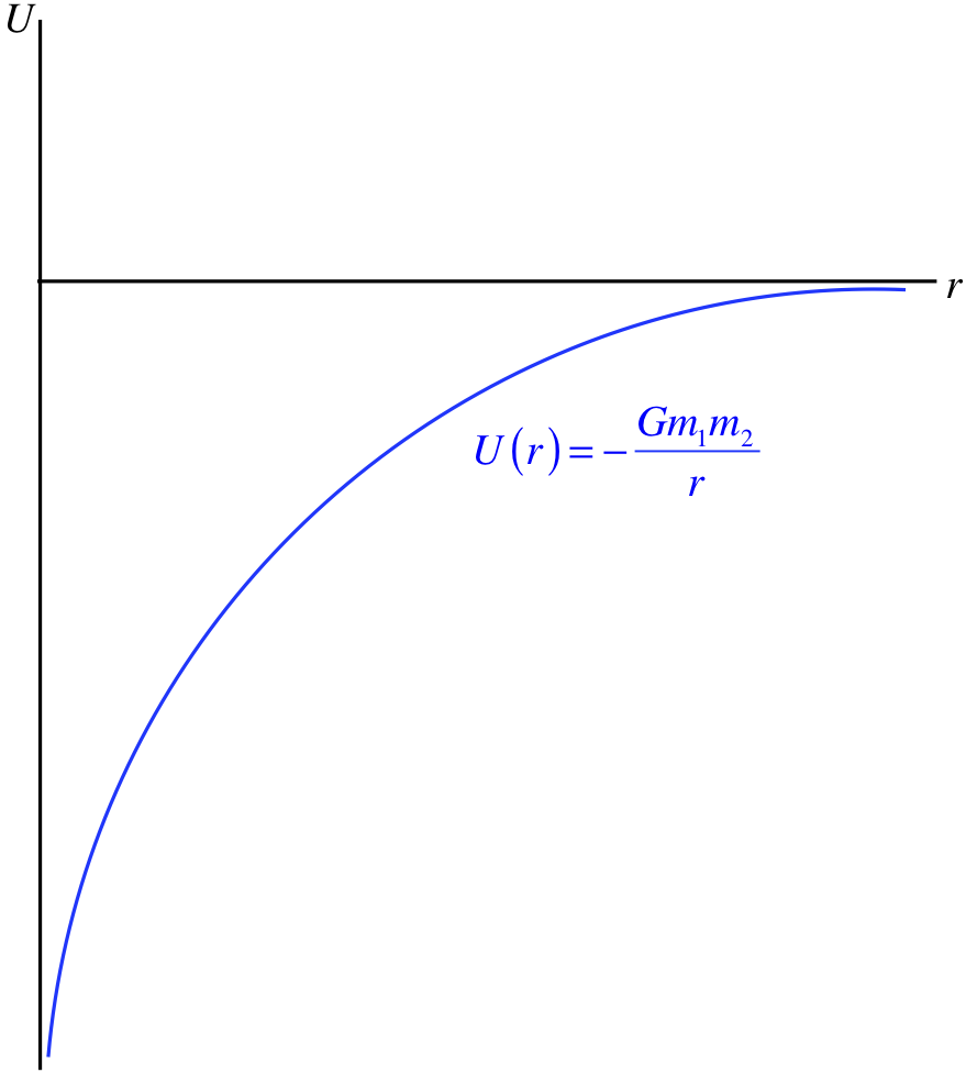
This function is significantly different from the "\(mgy\)" that we have been using up to now. To reconcile these two models, we need to make a note of the restriction of our terrestrial model of gravity – it holds for a region very close to the surface of the Earth, \(r=R_{Earth}\). Calling "\(h\)" the height of the object from the ground, the gravitational potential function above is cut-off at ground level. If we restrict ourselves to \(r\) values close to this point, the curve above is very close to a straight line:
Figure 7.3.2 – Gravitational Potential Near Earth's Surface
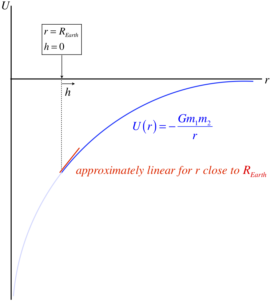
The negative slope of the potential energy curve is the force, so the slope of the straight line approximating the curve near \(r=R_{Earth}\) is the constant force in that region. Taking the negative derivative gives Newton's gravitational force, and when evaluated at \(r=R_{Earth}\), this force comes out to be \(mg\), as we saw in Equation 7.1.4.
Bound and Unbound Gravitational Systems
With a graph of the potential energy which goes to zero at infinity, we are naturally drawn again to energy diagrams. There is a problem with jumping straight into this, however. Energy diagrams require 1-dimensional motion, and while \(U\left(r\right)\) is a function of a single variable, the motion is not 1-dimensional. To see where things break down, consider a closed elliptical orbit. As the planet moves toward the perihelion, the value of \(r\) gets smaller. If Figure 7.3.1 were the potential curve for an energy diagram, then when the planet is moving toward smaller values of \(r\), it would keep speeding up indefinitely as it approaches \(r=0\). Okay, so in practice it would hit the surface of the sun before it could "accelerate indefinitely," but still this does not represent orbital motion. In short, there is no part of this potential energy graph that represents the turnaround point that is the perihelion.
Fortunately, we have a nice trick to take care of this shortcoming. When we draw energy diagrams, the kinetic energy comes from the motion along the direction parallel to the one dimension. In this case of measuring energy along the radius, the kinetic energy for the energy diagram can only come from the part of the velocity that is radial. The total kinetic energy is the sum of the radial and tangential parts:
\[ KE_{tot} = KE_{radial} + KE_{tangential} \]
The tangential speed multiplied by the mass and the distance from the center is the angular momentum, which is a constant of the motion, so we have:
\[ \left. \begin{array}{l} KE_{tangential} = \frac{1}{2}mv_{tangential}^2 \\ L = mv_{tangential}r \end{array} \right\} \;\;\; \Rightarrow \;\;\; KE_{tangential} = \dfrac{L^2}{2mr^2} \]
If we now construct the total energy of the system, we have:
\[ E_{tot} = KE_{radial} + KE_{tangential} + U = \frac{1}{2}mv_{radial}^2 + \dfrac{L^2}{2mr^2} - \dfrac{GMm}{r} \]
Note that this can now be treated as 1-dimensional system, by combining the last two terms into a single function of \(r\) that we call an effective potential:
\[ U_{eff}\left(r\right) = \dfrac{L^2}{2mr^2} - \dfrac{GMm}{r} \]
Graphing this allows us to work exactly as before, though we have to keep in mind that whatever we determine the kinetic energy to be is really only a fraction of the kinetic energy. So, for example, at the turnaround points (where we have said the kinetic energy is zero), the kinetic energy is in fact the tangential term. This makes sense for closed orbits, since the orbiting body never actually stops moving entirely – it only stops moving radially. The graph of this effective potential has a rather familiar shape, and including the total system energy makes it an energy diagram.
Figure 7.3.3 – Energy Diagram of a Gravitating System
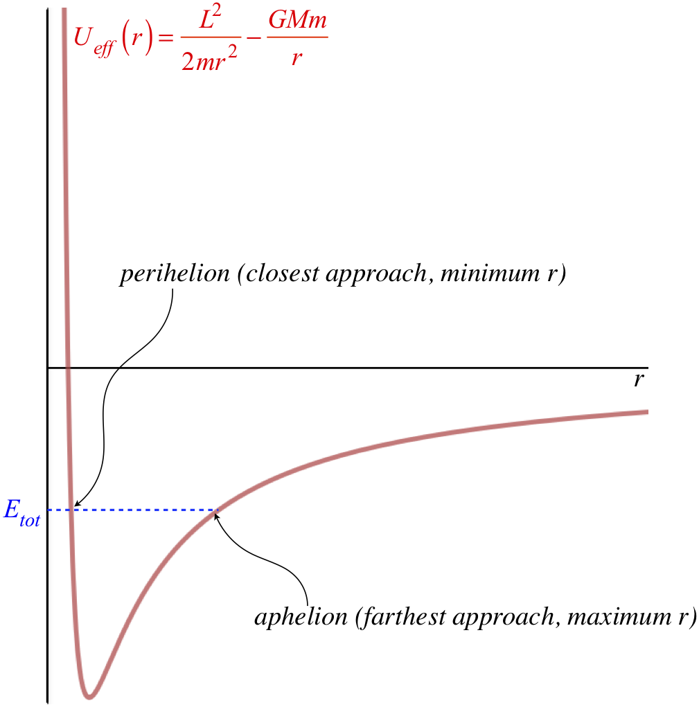
Figure 7.3.3 labels the turnaround points as the perihelion and aphelion, but there is much more we can extract from this diagram:
- circular motion
If the total energy lies at the bottom of the dip, then according to what we know about about energy diagrams, the kinetic energy is zero. But in this case, it means that the contribution to the kinetic energy by the radial component of velocity is zero. In other words, the orbit is circular. This fits with the fact that there is only one turnaround point, making the perihelion and aphelion the same distance.
- semi-major axis
The semi-major axis is the average of the perihelion and aphelion distances, so it is the value of \(r\) halfway between the two turnaround points on the graph.
- eccentricity
Looking at Figure 7.2.1, we can write the perihelion and aphelion distances in terms of the eccentricity and the semi-major axis, which we can then invert to get the eccentricity in terms of the perihelion and aphelion distances and the semi-major axis. Doing this gives:
\[ e = \dfrac{r_{max} - r_{min}}{2a} \]
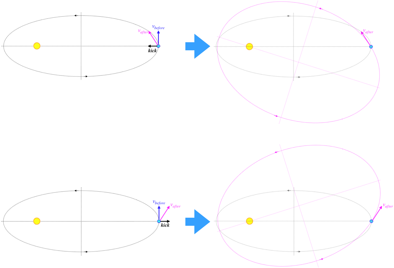
Looking at Figure 7.3.3, we see that raising the total energy (but keeping it negative, and doing it without increasing the angular momentum, which would change the graph) increases the length of the semi-major axis, but much more of this change comes from the increase of the aphelion distance than from the decrease of the perihelion distance (especially close to the horizontal axis). This results in an increase of eccentricity. How does one increase the total energy without increasing the angular momentum? By giving the orbiting body a "kick" that points radially (inward or outward). This exerts no torque (the force is parallel to the position vector), so the angular momentum doesn't change, but the push increases the total energy, because it adds a radial component of velocity without changing the tangential component.
When a radial kick is given, a polar angle of zero in the same coordinate system will no longer correspond to the aphelion of the orbit – the orbital ellipse will be rotated. If the kick is outward, then at the position of the kick the orbiting body is still getting farther from the gravitating body, which means it is heading for the new aphelion, and the orbit has rotated in the direction of the orbit. That is, if the orbit was clockwise, then the major axis rotates clockwise. For a radially inward kick, the orbiting body is now getting closer to the gravitating body, which means it is coming from the aphelion, so the major has rotated the direction opposite to the orbit direction.
Figure 7.3.4 – Effect of Radial "Kicks" to Orbits
A tangential kick in the direction of motion would also raise the total energy, but it would also increase the angular momentum, increasing the positive term in the effective potential. This has the effect of raising the bottom of the curve, and if this is done properly (at the aphelion), the bottom of the curve comes up faster than the energy line goes up, bringing the eccentricity down. The eccentricity can even be brought all the way down to zero (i.e. a circular orbit) in this way (see Example 7.3.1).
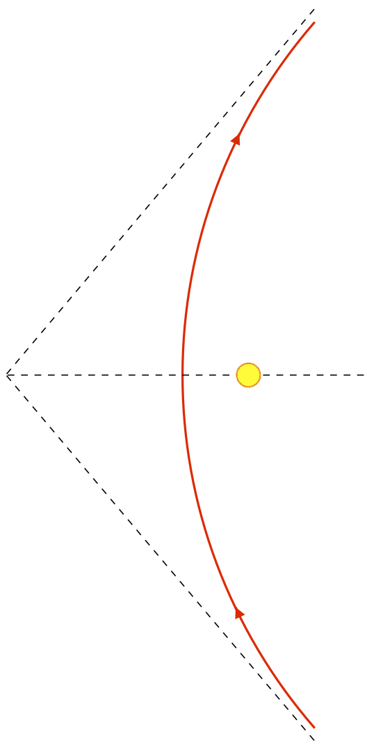
- hyperbolic trajectory – unbounded
If the total energy is greater than zero, the orbiting body is not "bound" to the gravitating body. That is, after the orbiting body makes its closest approach, it zooms away, and although it slows down as it departs, it never stops moving away from the gravitating body. The height of the total energy line above the horizontal axis represents the finite kinetic energy of the orbiting body when it gets very far away, since the potential vanishes there. While the tangential part of the kinetic energy also goes to zero very far away, the angular momentum does not vanish – it remains conserved. With a finite speed and a non-zero angular momentum, the motion of the orbiting body must be asymptotically approaching a line that passes by the gravitating body, and we get what is called a hyperbolic trajectory. [The word "trajectory" is generally preferred over "orbit," because the latter typically implies that the affected body is trapped by the gravitating body.]
The orbit equation that we found for the elliptical orbit (Equation 7.2.13) still works, but for the hyperbolic trajectory the eccentricity is greater than 1.
Figure 7.3.5 – Hyperbolic Trajectory
- parabolic trajectory – barely (un)bounded
If the total energy of the system equals exactly zero, then the orbiting body just barely runs out of velocity as it reaches infinity. It technically is neither bound nor unbound – it is at the borderline between the two. In this case, the eccentricity equals exactly 1.
An orbiting body is in an orbit where it is four times farther from the gravitating body at its aphelion than at its perihelion. By what percentage must its speed be increased at the aphelion to make its orbit circular?
- Solution
-
Since orbits are closed, if we instantaneously speed up the orbiting body at its aphelion, it will return to that same point with the same speed and moving in the same direction (i.e. its motion will still be perpendicular to the radius). That means that when the orbiting body returns, it will either be once again at its aphelion (if the speed was not increased substantially), or it will be at its perihelion (if the speed was increased a great deal). There is also an "in-between" increase whereby the perihelion and aphelion are the same – a circular orbit. We can compute the required increase in speed by comparing the speed at the aphelion of an eccentric orbit to the speed of a circular orbit whose radius is the same as the semi-major axis of the eccentric orbit. Starting with Equation 7.2.11, we have:
\[ v_{min} = \left(1-e\right)\dfrac{GMm}{L} = \left(1-e\right)\dfrac{GMm}{mv_{min}r_{max}} = \left(\dfrac{1-e}{1+e}\right)\dfrac{GM}{v_{min}a} \;\;\; \Rightarrow \;\;\; v_{min} = \sqrt{\left(\dfrac{1-e}{1+e}\right)\dfrac{GM}{a}} \nonumber \]
For a circular orbit, the eccentricity is zero, which makes the ratio of the minimum velocity of the eccentric and circular orbits:
\[ \dfrac{v_{circular}}{v_{min}} = \dfrac{\sqrt{\dfrac{GM}{R}}}{\sqrt{\left(\dfrac{1-e}{1+e}\right)\dfrac{GM}{a}}} = \sqrt{\left(\dfrac{1+e}{1-e}\right)\dfrac{a}{R}} \nonumber \]
The new circular orbit must have a radius equal to the aphelion distance of the previous orbit, so:
\[ \dfrac{v_{circular}}{v_{min}} = \sqrt{\left(\dfrac{1+e}{1-e}\right)\dfrac{a}{\left(1+e\right)a}} = \sqrt{\dfrac{1}{1-e}} \nonumber \]
Now we need to know the eccentricity for an orbit where the aphelion distance is 4 times the perihelion distance. Writing these distances in terms of the semi-major axis gives:
\[ \left. \begin{array}{l} r_{min} = \left(1-e\right)a \\ r_{max} = \left(1+e\right)a \end{array} \right\} \;\;\; \Rightarrow \;\;\; 4 = \dfrac{r_{max}}{r_{min}} = \dfrac{1+e}{1-e} \;\;\; \Rightarrow \;\;\; e=\frac{3}{5} \nonumber \]
Plugging this in above gives us that the velocity must be increased by a factor of \(\sqrt{\frac{5}{2}}\) at the aphelion of the eccentric orbit to turn it into a circular orbit. This corresponds to a percentage increase of:
\[ \%\;increase = \left(\sqrt{\frac{5}{2}}-1\right)\times 100\% = \boxed{58\%} \nonumber \]
Suppose an orbiting body is bound by the gravitational attraction of a gravitating body that is a distance \(R\) away. If it is bound, it must be that it possesses insufficient kinetic energy such that when it is added to the (negative) gravitational potential the total energy makes it to zero. We define escape velocity as the minimum speed that an orbiting body must have in order to (barely) go infinitely far away from a gravitational source. Setting the total energy equal to zero, for the case of the object moving at escape velocity, we have:
\[ \frac{1}{2}mv_{escape}^2 + U\left(R\right) = 0 \;\;\; \Rightarrow \;\;\; v_{escape} = \sqrt{-\dfrac{2U\left(R\right)}{m}} = \sqrt{\dfrac{2GM}{R}} \]
Notice that whether or not an object can escape a gravitational attraction doesn't depend upon the would-be escaper's mass, but only its velocity. This makes for an interesting discussion when it comes to light. Light has no mass, so we would think that Newton's law of gravitation would indicate that it is unaffected by gravity. But when it comes to escape velocity, the mass does not factor in at all, so is the conclusion that light is unaffected by gravity incorrect?
It turns out that in fact light is affected by gravity (and specifically how this happens requires Einstein's improved theory of gravity), but what is more, we can compute whether light can escape a gravitating body. The speed of light is a well-defined constant, so the question of whether light can escape boils down to how close the origination of the light is to the gravitating body, and of course the mass of that body. The distance from which light will not escape is known as the Schwarzschild radius, and is found by plugging the speed of light (typically designated as \(c\)) into the escape velocity formula:
\[ c = \sqrt{\dfrac{2GM}{R}} \;\;\; \Rightarrow \;\;\; R_S = \dfrac{2GM}{c^2} \]
The Earth's mass is \(5.97 \times 10^{24} kg\), and the speed of light is \(3.0 \times 10^{8} \frac{m}{s}\). Its Schwarzschild radius therefore comes out to equal about 8.8 millimeters. Okay, that is quite small, and since the distance is measured from the center of the Earth, it is clear that we will not witness the phenomenon of light being trapped by the Earth's gravity. For light to be trapped by gravity, the gravitating body must fall inside the Schwarzschild radius. This requires that the gravitating body be incredibly dense, and since the only force available to pull the matter into that kind of density is the same gravity force, generally a very large amount of mass is required. Assuming this occurs, the object thus created is called a black hole. This is a nicely descriptive name, as "black" indicates that light does not escape its gravitational influence. Explaining how appropriate the word "hole" is in this name requires some knowledge of Einstein's theory, which is unfortunately beyond the scope of this work.