
3.1: Vector Rotations


- Last updated
- Nov 8, 2022
- Save as PDF

( \newcommand{\kernel}{\mathrm{null}\,}\)
Active vs. Passive Rotations
We take a moment now away from relativity to explore more of the formalism related to vectors. In particular, we will be looking at changes to vectors that result in changing their directions while leaving their magnitudes intact – rotations.
In our dealings with vectors in Physics 9HA, we primarily dealt with vectors in terms of their components in a coordinate system, and we will continue with that practice here. The interesting thing about doing this is that this coordinate representation depends upon the choice of the coordinate axes along which the components are defined. That is, we can look at the same vector in two different coordinate systems, giving us different components for the same vector.
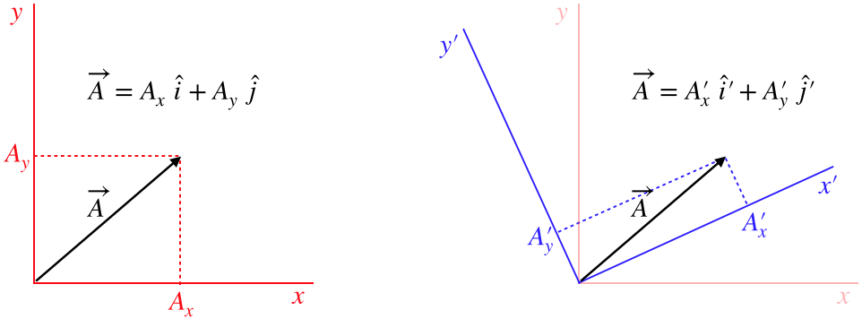
Figure 3.1.1 – Viewing the Same Vector in Two Coordinate Systems
Alert
It is worth emphasizing that we can only compare two vectors using their components if these components are measured on the same axes. Two vectors that are identical (i.e. represent the same physical quantity, giving us all the same experimental results, etc.) can be expressed entirely differently by their coordinates when different coordinate frames are used, so one must take care not to attribute too much "reality" to the components.
Looking at the diagram above, it's clear that the vector →A does not change orientation from one frame to the other – it is the same physical quantity whose components are measured with different axes – but if the people using these coordinate systems were to compare the angles they see this vector making with their respective x-axes, they would not agree. This might prompt them to say that the vector is "rotated" when going from one frame to the other. It isn't, of course, but we can express this mathematically as a coordinate transformation that looks like a rotation nonetheless. Such a transformation is called a passive rotation, to emphasize that the vector itself is not rotated.
Of course, vectors can also have their actual directions changed as well, such as a rock's velocity vector changing direction as it swings around a circle while tied to a string. These direction changes are due to some physical process, rather than a simple change of measurement perspective. When measured in the same coordinate system, these physical rotations are called active rotations.
Because both are typically expressed in terms of components, it is common to confuse active rotations for passive ones, so it is a good idea to keep in mind what is responsible for the rotation to keep them separate. In our study of relativity, our primary focus is on viewing physical quantities from different perspectives, so we will mainly deal with passive transformations in the sections to come. In order to avoid having to append the words "active" or "passive" every time we use the word "rotation," from this point forward we will assume that the rotation is passive unless explicitly stated otherwise.
Invariants
Rotations are defined by the fact that the magnitude of the vector doesn't change. We therefore declare the vector magnitude to be an invariant with respect to rotations. There are other invariants as well. The most trivial of these is the independent scalar (like the number 2), which has no connection to the orientation of spatial axes. One might be inspired to say, "The vector magnitude is a scalar, so of course it is an invariant!", but this logic is flawed. The x-component of a vector is also a scalar, but it changes when the coordinate system is rotated.
A vector-related quantity whose invariance may not be readily-apparent is the scalar product of two vectors. As stated above, we can't declare it an invariant simply because it is a scalar, and in fact when expressed in terms of coordinates, it is by no means obvious that the answer comes out the same in both coordinate systems:
→A⋅→B=AxBx+AyBy+AzBz?=A′xB′x+A′yB′y+A′zB′z
We will see how to write the primed coordinates in terms of the unprimed coordinates shortly, but we can resolve this issue without doing so by considering the other form of the dot product:
→A⋅→B=ABcosθ
Looking at this representation of the scalar product, we see that it depends upon the magnitudes of the two vectors, which we already know are invariant. Our passive rotation does not rotate the actual directions of either vector, so although the angles these vectors make with the axes change when the axes are rotated, the angle these two vectors make with each other doesn't change. With A, B, and θ all left unchanged by the rotation of the coordinate system, the scalar product remains unchanged, and is therefore invariant. Note that the magnitude-squared of a vector is simply a scalar product of the vector with itself (→A⋅→A=A2), so these two invariants are consistent with each other.
Transforming Vectors Between Rotated Frames
In keeping with our quest of expressing measurements made in one frame in terms of measurements made in another, we will examine the mathematics associated with translating between components of vectors measured by two coordinate systems rotated with respect to each other (called a rotational transformation between coordinate systems). We start by labeling quantities in Figure 3.1.1:
Figure 3.1.2 – Rotational Transformation
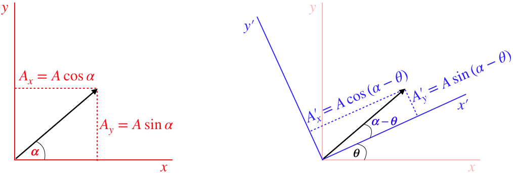
The primed coordinate axes have been rotated an amount θ in the positive (counterclockwise) direction relative to the unprimed coordinate axes. We can now write the components in the unprimed frame in terms of the angles α (the angle the vector makes in the unprimed frame) and θ using trigonometric identities for the difference of two angles:
To get the inverse transformation, we simply note that the red axes are rotated by the same angle θ relative to the blue axes, but in the opposite direction (clockwise), so simply making the change θ→−θ does the trick.
Example 3.1.1
Show the rotational transformation maintains the invariance of:
- the length of the vector
- the scalar product of two vectors
- Solution
-
a. Plugging the primed components into the pythagorean theorem and transforming them into unprimed components gives:
A2=A′2x+A′2y=(Axcosθ+Aysinθ)2+(−Axsinθ+Aycosθ)2=(A2xcos2θ+2AxAycosθsinθ+A2ysin2θ)+(A2xsin2θ−2AxAysinθcosθ+A2ycos2θ)=A2x(cos2θ+sin2θ)+A2y(sin2θ+cos2θ)=A2x+A2y
b. Plugging the primed components into the scalar product and transforming them into unprimed components gives:
→A⋅→B=A′xB′x+A′yB′y=(Axcosθ+Aysinθ)(Bxcosθ+Bysinθ)+(−Axsinθ+Aycosθ)(−Bxsinθ+Bycosθ)=(AxBxcos2θ+AxBycosθsinθ+AyBxsinθcosθ+AyBysin2θ)+(AxBxsin2θ−AxBysinθcosθ−AyBxcosθsinθ+AyBycos2θ)=AxBx(cos2θ+sin2θ)+AyBy(sin2θ+cos2θ)=AxBx+AyBy
A Bit About Matrices
Back in 9HA, we had an extremely brief encounter with column matrices as a tool for organizing the components of a vector. We will find these increasingly useful in our study of physics, starting with our current discussion of rotational transformations. By filling the rows of a column matrix with the components of a vector, we take for granted that each row represents one of the three axes. If we change our axes (say by rotating them), then each row means something different. So we need to come up with some mathematical procedure for changing the meaning of the rows. That is, we need to generate this change:
(component measured along x-axiscomponent measured along y-axiscomponent measured along z-axis)→ rotate axes →(component measured along x′-axiscomponent measured along y′-axiscomponent measured along z′-axis)
Note that this process represents a passive rotation, which means that although the two matrices have different entries, they represent the same vector. It's just that the matrix entries are associated with different axes. As we saw above, a component in one set of axes is expressed as a combination of more than one component in the other set of axes. We achieve this mathematically through matrix multiplication of a square matrix with the column matrix representing the vector:
(A′xA′yA′z)=(abclmnrst)(AxAyAz)
The way this multiplication works is this:
- grab the top row of the square matrix and rotate it clockwise by 90 degrees
- align the entries with those of the column matrix, and multiply corresponding entries
- add all of these products together
- place this sum at the top of a new column matrix
- repeat this process by moving to each subsequent row of the matrix, placing the resulting sum in the next row of the new column matrix
Figure 3.1.3 – Matrix Multiplication
Note that this only works when the number of columns of the square matrix matches the number of rows of the column matrix. Indeed more generally an m-by-n matrix (written "m×n", where m= number of rows, n= number of columns) can only multiply (from the left) an n×r matrix (where r is any positive integer), and the result is an m×r matrix. This is why transforming a column vector into another column vector requires a square matrix.
Let's put the rotation transformations in Equation 3.1.3 into matrix form. Noting that this rotation is around the z axis, so that the z coordinates don't change, we have:
(A′xA′yA′z)=(+cosθ+sinθ0−sinθ+cosθ0001)(AxAyAz)
The matrix that performs this rotation transformation between coordinate axes is called a rotation matrix. Keep in mind that this matrix simply helps us express the components of the same vector in a different set of coordinate axes that have (in this case) been rotated counterclockwise around the z-axis by an angle θ.
It's also useful to point out that the scalar product of two vectors can easily be expressed in terms of matrices if the first vector is expressed as a row (1×3) matrix, the second as a column (3×1) matrix, resulting in a scalar (1×1 matrix):
→A⋅→B=(AxAyAz)(BxByBz)=AxBx+AyBy+AzBz