4.1: Basics of Probability Theory

Probability Distributions 

Whenever we consider an outcome to a random event, the probability of that outcome is the ratio of its "measure" to the measure of all possible outcomes. Frequently this measure is computed purely by counting, and is particularly simple if each outcome is equally likely. Sometimes the counting is a bit more complicated, because the desired probability spans a group of distinguishable results. For example, if one asks for the probability of throwing a 7 on a standard pair of 6-sided dice, this "outcome" can occur in many ways: The first die can result in 1 and the second in 6, the first die 6 and the second 1, the first 5 and the second 2, and so on. There are 6 distinct rolls that result in this same outcome, giving it a measure of 6. The total number of possible rolls is the product of the number of possible results on the first die and the number of possible results on the second die, or 36. The ratio of the measure of the desired outcome to the measure of all outcomes is 6/36 = 1/6.

If the outcome of a roll of two dice is defined as the total on both dice, then all outcomes are not equally-probable. For example, there are more ways to roll a total of 6 (five ways) than a total of 5 (four ways). The map of probabilities for the various possible outcomes is called the probability distribution. For two dice, there are eleven possible outcomes, and the probability distribution for these outcomes are shown below.

Figure 4.1.1 – Probability Distribution for Sum of Two Six-Sided Dice

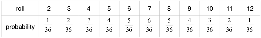
This probability distribution involves different probabilities for different outcomes. Those (like for the roll of a single die) that provide the same probability for all outcomes are called uniform. Quite often when one knows of no mechanism that would cause results to clump into certain outcomes, the first guess at the probability distribution is uniform. This assessment can change either with increased knowledge of the randomizing mechanism (e.g. a single die is found to be weighted unsymmetrically), or data indicating that the original assumption was likely bad (e.g. a single die comes up one number much more often than random chance would indicate).

Mutually-Exclusive Outcomes 

In the case of the roll of a pair of dice, clearly it is impossible to get both a 6 and an 8 on the same roll. The roll of a 8 excludes the possibility of the roll of an 8, and a roll of an 8 excludes the possibility of the roll of a 6.  Two outcomes of these kinds are referred to as mutually-exclusive.

If we enumerate all of the mutually-exclusive outcomes for a random event, the one and only one of them must occur. The possible rolls of two dice are the numbers 2 through 12. If we add up all of the probabilities for these outcomes, we get a sum equal to 1. We can ask what the probability is that the random event will result in either outcome A or outcome B. If these outcomes are mutually-exclusive, then the probability of one or the other occurring is the sum of the probabilities:

\[P\left(A~or~B\right)=P\left(A\right)+P\left(B\right)~~~~~\text{A and B mutually exclusive}\]

One must be very careful to only use this sum of probabilities under these restrictions. Not all probabilities that involve "or" is a simple sum.  For example, one could ask what the probability is that for a roll of two dice, the red die comes up 2, or the green die comes up 2.  The probability of a single die coming up 2 is \(\frac{1}{6}\), so one might guess that the probability of one or the other coming up 2 is \(\frac{1}{6}+\frac{1}{6}=\frac{1}{3}\), but it is not!  The roll of a 2 on the red die does not exclude the roll of a 2 on the green die. As these are not mutually-exclusive, you cannot add their probabilities.

Independent Outcomes 

The opposite case of mutually-exclusive outcomes are independent outcomes. As suggested by the name, two outcomes that are independent have no effect over one another. The case above of the 2 coming up on the red die and the 2 coming up on the green die is an example of two independent outcomes. As we saw above, we cannot sum probabilities for "or's" in these cases, but there is a parallel bit of math we can do.

When the dice are rolled, we can use the individual probabilities to compute the probability of both independent events occurring. This is a simple matter of multiplying the probabilities:

\[P\left(A~and~B\right)=P\left(A\right)\times P\left(B\right)~~~~~\text{A and B independent}\]

In the case of rolling 2's on both dice, the probability is the product of the two probabilities: \(\frac{1}{6}\times\frac{1}{6}=\frac{1}{36}\).

Note that this also makes it possible to properly compute the probability of a 2 on either the green or the red (or both).  We do this using the "and" property as follows: The probability that one die misses a 2 is \(\frac{5}{6}\), so the probability that both dice miss 2's is \(\frac{5}{6}\times\frac{5}{6}=\frac{25}{36}\). But if both dice missing 2's doesn't occur, then that means at least one of the dice is a 2. Since these two cases represent all the outcomes, the sum of their probabilities is 1, which means that the probability of the red die rolling a 2 or a green dies rolling a 2 (or both rolling 2's) is \(1-\frac{25}{36}=\frac{11}{36}\). Note that this is not quite equal to the \(\frac{1}{3}\) result found in the erroneous calculation earlier.

Expectation Values 

Where probabilities become particularly important is when the outcomes are accompanied by measurable results. Continuing with our pair of dice example, let's suppose that two people wager on the outcome of a roll. If the same wager is made over and over many times, the outcomes can be summed together and divided by the number of rolls to get an average outcome per roll.  This average of a single outcome need not be one of the possible outcomes of a single roll, but is referred to as the expectation value of a single event.

The way to use probabilities to compute expectation values is as follows: Multiply the probability of every outcome by the value of that outcome, and sum all of these products:

\[\left<\omega\right>=P\left(A\right)\cdot \omega\left(A\right)+P\left(B\right)\cdot \omega\left(B\right)+\dots\]

Let's look at an example of an expectation value for our dice roll model...

Ann and Bob agree that Ann will receive $4 from Bob if the result of a two-dice roll is a 4 or a 7, and Bob will receive $3 from Ann if the result is a 6 or an 8. Neither wins any money if anything else is rolled. Let's compute the expectation value of what Bob will receive per roll.  The results 4 and 7 are mutually-exclusive, so we can add their probabilities to get the probability of Bob winning: \(\frac{3}{36}+\frac{6}{36}=\frac{1}{4}\). The probability of Bob losing is similarly: \(\frac{5}{36}+\frac{5}{36}=\frac{5}{18}\). The remainder is the probability that no one wins: \(1-\frac{9}{36}-\frac{10}{36}=\frac{17}{36}\).  Now multiply these probabilities by the outcomes for Ann to get her expectation value:

\[\left<\omega\right>=\left(\frac{1}{4}\right)\left(+$4\right)+\left(\frac{5}{18}\right)\left(-$3\right)+\left(\frac{17}{36}\right)\left($0\right)=+\frac{1}{6}\left($1\right)\]