4.4: Physical Measurements with Random Outcomes

Probability Amplitude

We have discussed how light and matter both behave light particles and waves, and the fact that combining the wave nature with the observance individual dots on a screen leads us to the inescapable truth that nature behaves probabilistically on a fundamental level. We said this was because the interference pattern occurred even when we sent one particle at a time (i.e. we waited for the dot to appear before sending another particle), which means that regions with higher densities of dots must be more probable landing points than those with low densities of dots. Let's apply some of the tools of probability theory to the double-slit experiment in order to construct a mathematical model for what is happening.

We'll start by labeling a few parts of the double-slit experiment. We'll label a starting point of the electron or photon (the source of the beam) with an '\(i\)', and the eventual landing point (dot on the screen) with an '\(f\)'.  The two possible paths (slits) we will label with an '\(A\)' and a '\(B\)'.

Figure 4.4.1 – Defining Paths for a Particle Through a Double-Slit

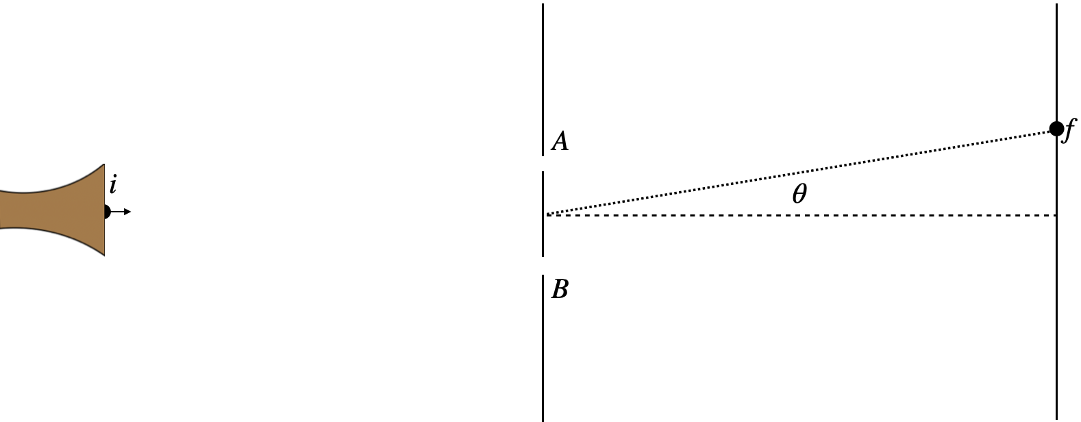
Returning to the idea that this particle has a localized nature (it makes dots on the screen), it seems reasonable to conclude that this dot either passed through slit \(A\) or through slit \(B\), and that these two choices are mutually exclusive. From what we know of probability theory (Equation 4.1.1), we can write the probability of getting from \(i\) to \(f\) as the sum of the probabilities of making this journey through slit \(A\) and through slit \(B\):

\[P\left(i\rightarrow f\right)=P\left(i\rightarrow A\rightarrow f\right)+P\left(i\rightarrow B\rightarrow f\right)=P_{\text{through A}}\left(\theta\right)+P_{\text{through B}}\left(\theta\right)\]

But if we close slit \(B\), the probability \(P\left(i\rightarrow A\rightarrow f\right)\) doesn't change. The only difference is that the particles that were previously going through slit \(B\) get blocked by the barrier we put there. So using this math leads to the incorrect prediction depicted in Figure 3.4.2.

The problem is with destructive interference. Probabilities (and probability densities) are always positive, so they cannot cancel each other, as these seem to do. So to explain this experiment, we must marry the purely-positive nature of probabilities with the potential for destructive interference. Well it turns out that we've had the idea for this all along! We found long ago two things:

1. The intensity pattern is directly related to the probability – the more densely-packed the dots are in a region of the screen, the higher the probability must be that a single particle will land in the region.
2. Intensity of a wave is proportional to the square of its amplitude.

We therefore infer the existence of a probability amplitude. This is the amplitude of the wave (whether it is an EM wave or a matter wave), that can interfere with itself in a double-slit apparatus.  The phase of the wave can turn this amplitude into a positive or negative (or actually, as we will see later, a complex) quantity, which allows it to result in destructive interference. The square of this value (which becomes a bit more complicated when we get to complex-valued amplitudes) is the probability density, which remains strictly positive, as it must.

Because of the principle of superposition of waves, these probability amplitudes (adjusted by the phases of their associated waves) are the quantities that we add for the two paths, rather than the probabilities. The paths are not mutually exclusive – the wave passes through both slits, not strictly one or the other. If we call the wave that arrives at \(f\) (deflects through \(\theta\)) from \(i\) through slit \(A\) '\(\psi_A\left(\theta\right)\)' and the wave that goes through slit \(B\) '\(\psi_B\left(\theta\right)\)', then the total wave is:

\[\psi_{tot}\left(\theta\right)=\psi_A\left(\theta\right)+\psi_B\left(\theta\right)\]

The probability density at that position on the screen is then the square of this total (in anticipation of these probability amplitudes being complex, we'll use the proper description of these squares here, but don't worry about this notation yet):

\[\mathcal P\left(\theta\right)=\left|\psi_{tot}\left(\theta\right)\right|^2=\left|\psi_A\left(\theta\right)+\psi_B\left(\theta\right)\right|^2=\left|\psi_A\left(\theta\right)\right|^2+\left|\psi_B\left(\theta\right)\right|^2+2\psi_A^*\left(\theta\right)\psi_B\left(\theta\right)\]

The last term here is where there is potential for negative numbers. If not for this "overlap" term, then the mutually-exclusive assumption would be correct.

Summarizing the Path from Physical Properties to Probabilistic Predictions

We have now seen three different quantities that include the word "probability" in their names, and it is useful to have a look back to make sure we have them straight, and clarify how they fit into the physics.  We will do this by outlining the steps of how we "do" quantum physics...

• Physical features of the system are determined. These are things like the separation of two slits, the gap sizes of each slit, directions of polarization of polaroids, electrical forces on charged particles, etc.
• The physical features have an effect on the wave function and its boundary conditions.
• Use superposition of wave functions to obtain a single probability amplitude:

\[\psi_{tot}\left(x\right)=\psi_1\left(x\right)+\psi_2\left(x\right)+\dots\]

• Square the probability amplitude to get the probability density:

\[\mathcal P\left(x\right)=\left|\psi_{tot}\left(x\right)\right|^2\]

• Use the probability density over a range of values to obtain the probability that a value lands in a range:

\[P\left(x\leftrightarrow dx\right)=\mathcal P\left(x\right)dx=\left|\psi_{tot}\left(x\right)\right|^2dx\]

• Use the probability density to compute expectation values and uncertainties of physically-measurable quantities:

\[\left<\omega\right>=\int\limits_{-\infty}^{+\infty}\omega\left(x\right)\left|\psi_{tot}\left(x\right)\right|^2dx\]

Of course there are many details left out here, the most notable being the grief and heartache that goes into finding the wave function from the physical conditions. But there are also mathematical details to keep in mind, such as making sure that the probability density is normalized and a few other things we will discuss soon. But this outlines the main procedure we will follow.

Observables Other than Position

So far we have focused only on the probabilistic nature of measurement of position, but this is certainly not the only observable for which quantum mechanics provides randomness. We have so far only dealt with matter and light with a single wavelength (in one dimension, these are plane waves). Such quanta will not result in a probabilistic measure of momentum or kinetic energy – a single wavelength means a single value for these quantities. But as we noted all the way back in Equation 1.1.16 (and used over and over since then, most notably in Fourier analysis), a solution to the wave equation can be linear combination of many waves, which can all have different wavelengths. This means that the wave function of a single quanta can actually be a linear combination of many single-wavelength waves. If the particle is confined, then its wave is a standing wave, and is a sum of single wavelength harmonics (i.e. is a Fourier series). But even if it is free from confinement, its wave can be a mix of waves of many wavelengths.

What would the momentum of such a particle be, if its de Broglie wavelength is not uniquely-defined? That's exactly the point – it has no specific momentum! We can of course make a measurement of such a particle's momentum, and we will get a value that is associated with one of the many wavelengths that make up this wave. The wavelength that gets chosen from the collection is selected at random, and each wavelength has its own probability of being selected. Momentum (and with it, kinetic energy) is – like position – determined probabilistically!

Dirac Brackets Again

We return now to those enigmatic bras and kets that first appeared in Section 1.6 and later made a brief appearance in Section 3.5. We said that the quantity \(\left|\psi\right>\) is an abstract vector that contains all the information of the quantum state, and that we can extract this information from it by taking "dot products". Now we have the language to put this together. Suppose we wish to know the probability that the particle in the quantum state \(\left|\psi\right>\) will be found to be at position \(x\). The quantum state of being precisely at \(x\) (i.e. seeing the dot on a screen at \(x\)), we define as \(\left<x\right|\). The full quantum state of the particle includes the possibility of the particle being anywhere, but the dot product of this full state with the precise state of location at \(x\) is the probability amplitude of the particle being found there:

\[\text{probability amplitude of measuring particle's position to be}~x=\left<x|\psi\right>\]

Given that there is a separate value of this probability amplitude at every position, this can be written as a function (a wave function), as we already stated in Equation 3.5.1:

\[\left<x|\psi\right>=\psi\left(x\right)\]

But this doesn't only apply to position! The quantum state vector also contains information about quantities like momentum. The quantum state of a particle having a precise momentum (which we know manifests as a single-wavelength wave) we will call \(\left<p|\psi\right|\). Then the probability amplitude of measuring the particle's momentum to be \(p\) is:

\[\text{probability amplitude of measuring particle's momentum to be}~p=\left<p|\psi\right>=\phi\left(p\right)\]

[Note: While not strictly necessary since the context is usually clear, it is traditional to use a different symbol for a wave function expressed with momenta than is used for positions.  So we will typically use \(\psi\left(x\right)\) and \(\phi\left(p\right)\).]

All of the same machinery we developed for calculating probabilities for positions applies equally to wave functions written in terms of momentum.  That is, the probability of measuring a particle's momentum to be between \(p_1\) and \(p_2\) is:

\[P\left(p_1<p<p_2\right)=\int\limits_{p_1}^{p_2}\left|\phi\left(p\right)\right|^2dp\]

And the expectation value of momentum is:

\[\left<p\right>=\int\limits_{-\infty}^{+\infty}p~\left|\phi\left(p\right)\right|^2dp\]

We get a nice bonus in the case of momentum, in that we also get kinetic energy, since \(KE=\frac{p^2}{2m}\):

\[\left<KE\right>=\int\limits_{-\infty}^{+\infty}KE~\left|\phi\left(p\right)\right|^2dp=\frac{1}{2m}\int\limits_{-\infty}^{+\infty}p^2~\left|\phi\left(p\right)\right|^2dp=\frac{1}{2m}\left<p^2\right>\]

What About Time?

The reader may be wondering about what happened to the time element for waves – aren't wave functions supposed to look like "\(f\left(x,t\right)\)"? Yes, of course! We got away from worrying about the time portion of the wave function because we were discussing static interference patterns. Although the wave function that results in a double-slit pattern evolves with time, the result itself comes out to be time-independent, so we were able to ignore the effect of the time contribution. As it turns out, we will be able to do this quite a lot in the chapters to come, largely because of the separation of variables trick we first discussed in Section 1.2.

But there is another aspect of this that should not be overlooked. An interference pattern is often not static. For example, a standing wave on a string is certainly not static – the string vibrates with time! But when it comes to probability amplitude, it is exactly that – the amplitude – that contributes to the critical probability density. Aside from the nodes, every point on a string with a standing wave harmonic is moving, but all of these points have amplitudes that are constants in time. The position of that piece of string is changing, but its amplitude (its maximum displacement) remains constant when the standing wave is a harmonic. It is this amplitude that comes into play in quantum probabilities, so even though the wave function may be changing with time, the probabilities associated with different positions may remain fixed. We will later see what physical properties must exist for this to be true.