4.2: Continuous Probability Distributions and Probability Density

Infinite Number of Outcomes

There is no reason why all probability distributions must be discrete as it is for two dice. Probability distributions on a continuum are also possible. The probability of a blindfolded dart thrower hitting various positions on a dart board could be an example of a two-dimensional continuous probability distribution.

The key feature of probability on a continuum is that one can no longer say that a given outcome has a specific probability.  If one selects a number at random from 0 to 1, the probability of hitting exactly a predicted number is zero, as there are uncountably-many choices. Even though one of those numbers is selected, its probability of being correctly-guessed was zero.

In such cases where the outcomes lie on a continuum, we need a different way to express probabilities – we need to express them in a range. So rather than talk about the probability of an outcome being exactly equal to \(x\), we define a probability of lying between \(x_1\) and \(x_2\). If the probability density on the continuum is uniform, then the calculation of the probability of lying within a range is easy. If, for example, all the outcomes of a random number lie on a number line between 0 and 8, then the probability of a single outcome occurring between 1.2 and 3.6 is the ratio of the size of the target range and the size of the full range: \(P\left(1.2\leftrightarrow 3.6\right)=\frac{3.6-1.2}{8}=0.3\).

But what if the probability distribution is not uniform, that is, what if the outcomes at some places in the continuum are more probable than others?

Probability Density

If we have a continuous probability distribution (of any dimension), then the measure for any individual result is actually zero, as there are infinitely-many possible outcomes. However, this doesn't make all the outcomes equally likely, because they may have different relative measures. For example, if the probability of one outcome is \(P\) and the probability of a second outcome is \(3P\), then the ratio of these outcomes shows that the latter outcome is three times more likely than the former, even in the limit as \(P\) goes to zero. Also, the sum of the infinite number of zero-probability outcomes still must equal one. We assure that this works properly by representing the continuous probability distribution with a probability density function.

As with any other density function we have encountered (such as mass density), the idea is to measure the relative weightings at various positions. For a line of mass along the \(x\)-axis with a mass density of \(\lambda\left(x\right)\), the infinitesimal amount of mass found in the tiny slice between positions \(x\) and \(x+dx\) is given by \(dm=\lambda\left(x\right)dx\).

Figure 4.2.1 Amount of Mass In an Infinitesimal Section in Terms of Density

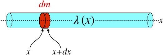
Now imagine that instead of a line of matter with varying mass density, we were talking about a particle bouncing back-and-forth within an opaque tube. The particle could be anywhere within the tube, and its probability of being between \(x\) and \(x+dx\) is infinitesimally small. But we can describe the probability of it being in that region in terms of the probability density function \(\mathcal P\left(x\right)\) in the same way as we did for mass:

\[dP\left(x\leftrightarrow x+dx\right) = \mathcal P\left(x\right)dx \]

Then the probability of it lying within a finite range is just the sum (the outcomes are mutually-exclusive) of all of these infinitesimal probabilities:

\[P\left(x_1\leftrightarrow x_2\right)=\int\limits_{x_1}^{x_2}dP=\int\limits_{x_1}^{x_2}\mathcal P\left(x\right)dx\]

Normalization

A universal truth of probability theory is that when the result of a random event occurs, it must land within the universe of possible outcomes. Mathematically, this means that the sum of the probabilities of all possible outcomes must be 1. This can be confirmed for the case of the roll of two 6-side dice by summing all of the probabilities in Figure 4.1.1.

What distinguishes the various probabilities from each other are their relative measures. In the example of the two dice, the probability of throwing a 7 is twice as great as throwing a 4 or a 10. We can determine these measures by comparing the number of ways the results can occur (six ways for the 7 versus three ways for the 4 and 10), but if we want to be able to properly use the probability distribution, we must divide all these measures by the sum of all measures so that the new sum is 1. This process is called normalization.

Imposing the normalization condition on a probability density function requires that:

\[1=\int\limits_{\text{all }x}\mathcal P\left(x\right)dx\]

In the work that follows, '\(x\)' will usually (but not always!) refer to an actual position in a one-dimensional space, so "integrating over all \(x\)" means that the normalization condition is typically:

\[1=\int\limits_{-\infty}^{+\infty}\mathcal P\left(x\right)dx\]

Expectation Value

To complete our extension of the previous section to the case of a continuum of outcomes, we have to address expectation values. If there are infinitude of possible outcomes because they are distributed on a continuum, then the sum given in Equation 4.1.3 is a sum of the product of the infinitesimal outcome probabilities multiplied by the values for each of the outcomes:

\[ \left<\omega\right> =\int \limits_{-\infty}^{+\infty}\mathcal P\left(x\right)\omega\left(x\right)dx \]

It is important to note that the expectation value is, in statistics terms, the mean of the distribution (as opposed to the mode and median, two other statistical measures of the "center" of a distribution), which means that like the discrete case, this value is not necessarily one of the possible outcomes.

Example \(\PageIndex{1}\)

A block vibrates on a frictionless horizontal surface while attached to a spring with spring constant \(k\). The maximum distance that the mass gets from the equilibrium point is \(x_o\). A radar gun measures the speed of the block at many random times, and these speeds are combined with the mass of the block to compute the block's kinetic energy. Find the average kinetic energy measured.

Solution

There are several ways to approach this. We will take the brute-force method here, to emphasize the mathematical details of the probability density integral. We start by determining the probability of the block being between \(x\) and \(x+dx\) at any random moment (with \(x\) measured from the equilibrium point of the spring). First, it should be clear that the probability density is not uniform – the block spends longer near the extreme ends of the oscillation than near the center, because it is moving slower near the endpoints. The probability of being in the tiny range \(dx\) will be the ratio of the time it spends there (which we'll call \(dt\)) to the time it spends going from one end of the oscillation to the other (half a period, \(\frac{1}{2}T\)):

\[P\left(x\right)dx = \dfrac{dt}{\frac{1}{2}T} \;\;\; \Rightarrow \;\;\; P\left(x\right)=\left(\dfrac{2}{T}\right)\dfrac{dt}{dx} = \dfrac{2}{vT} \nonumber\]

Plugging this into the expectation value equation for kinetic energy gives:

\[ \left<KE\right> = \int \limits_{-x_o}^{+x_o} P\left(x\right)\left[\frac{1}{2}mv^2\right]dx = \dfrac{m}{T}\int \limits_{-x_o}^{+x_o} v\;dx \nonumber \]

Clearly the velocity of the block changes with respect to \(x\), so \(v\) cannot be pulled out of the integral. The function of \(x\) that we plug in to \(v\) is found by noting that the total energy of the system remains constant, and equals the potential energy at the extreme points of the oscillation:

\[E=\frac{1}{2}mv^2+\frac{1}{2}kx^2= \frac{1}{2}kx_o^2\;\;\; \Rightarrow \;\;\; v\left(x\right) = x_o\sqrt{\dfrac{k}{m}}\sqrt{1-\left(\frac{x}{x_o}\right)^2} \nonumber\]

Plugging this into the integral and making the substitution \(u \equiv \frac{x}{x_o}\) gives:

\[ \left<KE\right> = \dfrac{mx_o^2}{T}\sqrt{\dfrac{k}{m}}\int \limits_{-1}^{+1} \sqrt{1-u^2}du \nonumber \]

The reader that wants to do every step of the math can perform the integral with a trig substitution, but looking it up is also fine – it comes out to equal \(\frac{\pi}{2}\). All that remains is to use the period of oscillation for this simple harmonic oscillator in terms of the mass and spring constant:

\[ T=2\pi\sqrt{\dfrac{m}{k}} \;\;\; \Rightarrow \;\;\; \left<KE\right> = \frac{1}{4}kx_o^2 \nonumber \]

Note that the average kinetic energy is half the total energy, which means the average potential energy is the same – on average the energy is split evenly between the two modes.