4.1: Nuclear Shell Model

The simplest of the single particle models is the nuclear shell model. It is based on the observation that the nuclear mass formula, which describes the nuclear masses quite well on average, fails for certain “magic numbers”, i.e., for neutron number $N=20,28,50,82,126$ and proton number $Z=20,28,50,82$, as shown previously. These nuclei are much more strongly bound than the mass formula predicts, especially for the doubly magic cases, i.e., when $N$ and $Z$ are both magic. Further analysis suggests that this is due to a shell structure, as has been seen for electrons in atomic physics.

Mechanism that causes Shell Structure

So what causes the shell structure? In atoms it is the Coulomb force of the heavy nucleus that forces the electrons to occupy certain orbitals. This can be seen as an external agent. In nuclei no such external force exits, so we have to find a different mechanism.

The solution, and the reason the idea of shell structure in nuclei is such a counter-intuitive notion, is both elegant and simple. Consider a single nucleon in a nucleus. Within this nuclear fluid we can consider the interactions of each of the nucleons with the one we have singled out. All of these nucleons move rather quickly through this fluid, leading to the fact that our nucleons only sees the average effects of the attraction of all the other ones. This leads to us replacing, to first approximation, this effect by an average nuclear potential, as sketched in Figure $\PageIndex{1}$.

Figure $\PageIndex{1}$: A sketch of the averaging approximation

Thus the idea is that the shell structure is caused by the average field of all the other nucleons, a very elegant but rather surprising notion!

Modelling the Shell Structure

Whereas in atomic physics we solve the Coulomb force problem to get the shell structure, we expect that in nuclei the potential is more attractive in the centre, where the density is highest, and less attractive near the surface. There is no reason why the attraction should diverge anywhere, and we expect the potential to be finite everywhere. One potential that satisfies these criteria, and can be solved analytically, is the Harmonic oscillator potential. Let us use that as a first model, and solve

$$-\frac{\hbar^2}{2m}{\Delta} \psi({\vec{r}}) + \frac{1}{2} m \omega^2 r^2 \psi({\vec{r}}) = E \psi({\vec{r}}). \nonumber$$

The easiest way to solve this equation is to realize that, since $r^2 = x^2+y^2+z^2$, the Hamiltonian is actually a sum of an $x$, $y$ and $z$ harmonic oscillator, and the eigenvalues are the sum of those three oscillators,

$$E_{n_xn_yn_z} = (n_x+n_y+n_z +3/2)\hbar\omega. \nonumber$$

The great disadvantage of this form is that it ignores the rotational invariance of the potential. If we separate the Schrödinger equation in radial coordinates as $$R_{nl}(r)Y_{LM}(\theta,\phi) \nonumber$$ with $Y$ the spherical harmonics, we find

$$-\frac{\hbar^2}{2m}{\frac{1}{r^2}}\frac{\partial}{\partial r}\left(r^2 \frac{\partial}{\partial r}R(r) \right) + \frac{\hbar^2 L(L+1)}{r^2} R(r) + \frac{1}{2} m \omega^2 r^2 R(r) = E_{nL} R(r). \nonumber$$

In this case it can be shown that

$$E_{nL} = (2n+L+3/2) \hbar \omega, \nonumber$$

and $L$ is the orbital angular momentum of the state. We use the standard, so-called spectroscopic, notation of $s,p,d,f,g,h,i,j,\ldots$ for $L=0,1,2,\ldots$.

Figure $\PageIndex{2}$: A schematic representation of the shell structure in nuclei.

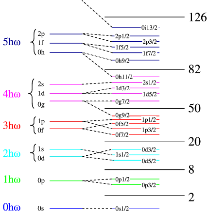
In the left hand side of Figure $\PageIndex{2}$ we have list the number harmonic oscillator quanta in each set of shells. We have made use of the fact that in the real potentials state of the same number of quanta but different $L$ are no longer degenerate, but there are groups of shells with big energy gaps between them. This cannot predict the magic numbers beyond 20, and we need to find a different mechanism. There is one already known for atoms, which is the so-called spin orbit splitting. This means that the degeneracy in the total angular momentum ($j=L\pm1/2$) is lifted by an energy term that splits the aligned from anti-aligned case. This is shown schematically in the right of the figure, where we label the states by $n$, $l$ and $j$. The gaps between the groups of shells are in reality much larger than the spacing within one shell, making the binding-energy of a closed-shell nucleus much lower than that of its neighbours.

Evidence for shell structure

Evidence for the shell structure can be seen in two ways:

1. By looking at nuclear reactions that add a nucleon or remove a nucleon from a closed shell nucleus. The most sensitive of these are electron knockout reactions, where an electron comes in and an electron and a proton or neutron escapes, usually denoted as ($e,e'p$) ($e,e'n$) reactions. In those we see clear evidence of peaks at the single particle energies.
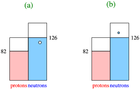
2. By looking at nuclei one particle or one hole away from a doubly magic nucleus. As an example look at the nuclei around $\ce{^{208}Pb}$, as in Figure $\PageIndex{3}$.

Figure $\PageIndex{3}$: The spectra for the one-neutron hole nucleus $^{207}$Pb and the one-particle nucleus $^{209}$Pb.

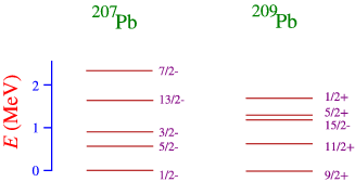
In order to understand this figure we need to think a little about the shell structure, as sketched very schematically in Figure $\PageIndex{4}$: The one neutron-hole nucleus corresponds to taking away a single neutron from the 50-82 shell, and the one neutron particle state to adding a neutron above the $N=128$ shell closure. We can also understand more clearly why a closed shell nucleus has very few low-energy excited quantum states, since we would have to create a hole below the closed shell, and promote the nucleon in that shell to an open state above the closure. This requires an energy that equals the gap in the single-particle energy.

Figure $\PageIndex{4}$: The shell structure of the one-neutron hole nucleus $^{207}$Pb and the one-particle nucleus $^{209}$Pb.