
6.2: The Schwarzschild Metric (Part 1)
- Page ID
- 11482

We now set ourselves the goal of finding the metric describing the static spacetime outside a spherically symmetric, nonrotating, body of mass m. This problem was first solved by Karl Schwarzschild in 1915.3 One byproduct of finding this metric will be the ability to calculate the geodetic effect exactly, but it will have more far-reaching consequences, including the existence of black holes. The problem we are solving is similar to calculating the spherically symmetric solution to Gauss’s law in a vacuum. The solution to the electrical problem is of the form \(\dfrac{\hat{\textbf{r}}}{r^{2}}\), with an arbitrary constant of proportionality that turns out to be proportional to the charge creating the field. One big difference, however, is that whereas Gauss’s law is linear, the equation
\[R_{ab} = 0\]
is highly nonlinear, so that the solution cannot simply be scaled up and down in proportion to \(m\).
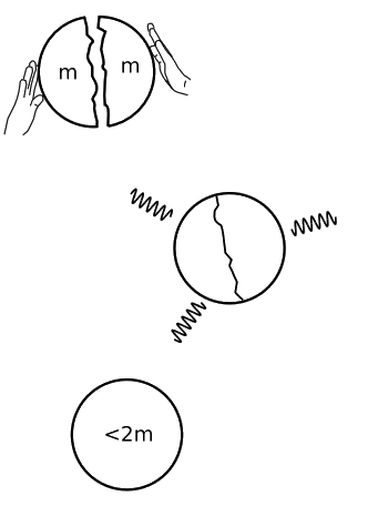
The reason for this nonlinearity is fundamental to general relativity. For example, when the earth condensed out of the primordial solar nebula, large amounts of heat were produced, and this energy was then gradually radiated into outer space, decreasing the total mass of the earth. If we pretend, as in Figure \(\PageIndex{1}\), that this process involved the merging of only two bodies, each with mass m, then the net result was essentially to take separated masses m and m at rest, and bring them close together to form close-neighbor masses m and m, again at rest. The amount of energy radiated away was proportional to m2, so the gravitational mass of the combined system has been reduced from \(2m\) to \(2m−(. . .)m^2\), where . . . is roughly \(\dfrac{G}{c^{2} r}\). There is a nonlinear dependence of the gravitational field on the masses.
Exercise \(\PageIndex{1}\)
The signature of a metric is defined as the list of positive and negative signs that occur when it is diagonalized.4 The equivalence principle requires that the signature be + − −− (or − + ++, depending on the choice of sign conventions). Verify that any constant metric (including a metric with the “wrong” signature, e.g., 2+2 dimensions rather than 3+1) is a solution to the Einstein field equation in vacuum.
4 See section 6.3 for a different but closely related use of the same term.
The correspondence principle tells us that our result must have a Newtonian limit, but the only variables involved are m and r, so this limit must be the one in which \(\dfrac{r}{m}\) is large. Large compared to what? There is nothing else available with which to compare, so it can only be large compared to some expression composed of the unitless constants G and c. We have already chosen units such that \(c = 1\), and we will now set \(G = 1\) as well. Mass and distance are now comparable, with the conversion factor being \(\dfrac{G}{c^{2}} = 7 \times 10^{−28} \,m/kg\), or about a mile per solar mass. Since the earth’s radius is thousands of times more than a mile, and its mass hundreds of thousands of times less than the sun’s, its \(\dfrac{r}{m}\) is very large, and the Newtonian approximation is good enough for all but the most precise applications, such as the GPS network or the Gravity Probe B experiment.
The Zero-mass Case
First let’s demonstrate the trivial solution with flat spacetime. In spherical coordinates, we have
\[ds^{2} = dt^{2} - dr^{2} - r^{2} \theta^{2} - r^{2} \sin^{2} \theta d \phi^{2} \ldotp\]
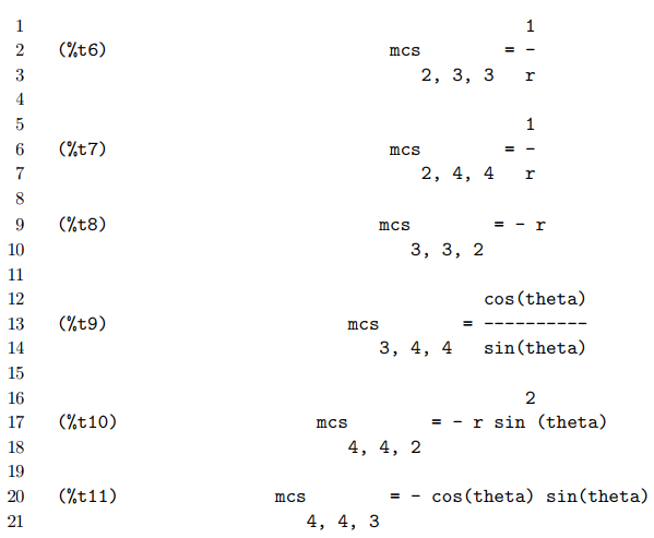
The nonvanishing Christoffel symbols (ignoring swaps of the lower indices) are:
\[\begin{split} \Gamma^{\theta}_{r \theta} &= \dfrac{1}{r} \\ \Gamma^{\phi}_{r \phi} &= \dfrac{1}{r} \\ \Gamma^{r}_{\theta \theta} &= -r \\ \Gamma^{r}_{\phi \phi} &= -r \sin^{2} \theta \\ \Gamma^{\theta}_{\phi \phi} &= \sin \theta \cos \theta \\ \Gamma^{\phi}_{\theta \phi} &= \cot \theta \end{split}\]
Exercise \(\PageIndex{2}\)
If we’d been using the (− + ++) metric instead of (+ − −−), what would have been the effect on the Christoffel symbols? What if we’d expressed the metric in different units, rescaling all the coordinates by a factor k?
Use of c tensor
In fact, when I calculated the Christoffel symbols above by hand, I got one of them wrong, and missed calculating one other because I thought it was zero. I only found my mistake by comparing against a result in a textbook. The computation of the Riemann tensor is an even bigger mess. It’s clearly a good idea to resort to a computer algebra system here. Cadabra, which was discussed earlier, is specifically designed for coordinate-independent calculations, so it won’t help us here. A good free and open-source choice is ctensor, which is one of the standard packages distributed along with the computer algebra system Maxima, introduced in section 2.5.
The following Maxima program calculates the Christoffel symbols found earlier.
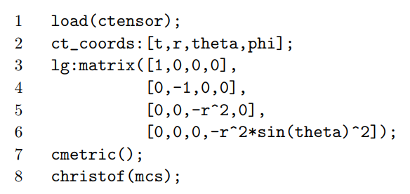
Line 1 loads the ctensor package. Line 2 sets up the names of the coordinates. Line 3 defines the gab, with 1g meaning “the version of g with lower indices.” Line 7 tells Maxima to do some setup work with gab, including the calculation of the inverse matrix gab, which is stored in ug. Line 8 says to calculate the Christoffel symbols. The notation mcs refers to the tensor \(\Gamma'^{a}_{bc}\) with the indices swapped around a little compared to the convention \(\Gamma^{a}_{bc}\) followed in this book. On a Linux system, we put the program in a file flat.mac and run it using the command maxima -b flat.mac. The relevant part of the output is:
Adding the command ricci(true); at the end of the program results in the output THIS SPACETIME IS EMPTY AND/OR FLAT, which saves us hours of tedious computation. The tensor ric (which here happens to be zero) is computed, and all its nonzero elements are printed out. There is a similar command riemann(true); to compute the Riemann rensor riem. This is stored so that riem[i,j,k,l] is what we would call Rlikj. Note that l is moved to the end, and j and k are also swapped.
Geometrized Units
If the mass creating the gravitational field isn’t zero, then we need to decide what units to measure it in. It has already proved very convenient to adopt units with \(c = 1\), and we will now also set the gravitational constant \(G = 1\). Previously, with only c set to 1, the units of time and length were the same, [T] = [L], and so were the units of mass and energy, [M] = [E]. With G = 1, all of these become the same units:
\[ [T] = [L] = [M] = [E].\]
Exercise \(\PageIndex{3}\)
Verify this statement by combining Newton’s law of gravity with Newton’s second law of motion.
The resulting system is referred to as geometrized, because units like mass that had formerly belonged to the province of mechanics are now measured using the same units we would use to do geometry.
A Large-r Limit
Now let’s think about how to tackle the real problem of finding the non-flat metric. Although general relativity lets us pick any coordinates we like, the spherical symmetry of the problem suggests using coordinates that exploit that symmetry. The flat-space coordinates \(\theta\) and \(\phi\) can stil be defined in the same way, and they have the same interpretation. For example, if we drop a test particle toward the mass from some point in space, its world-line will have constant \(\theta\) and \(\phi\). The r coordinate is a little different. In curved spacetime, the circumference of a circle is not equal to 2\(\pi\) times the distance from the center to the circle; in fact, the discrepancy between these two is essentially the definition of the Ricci curvature. This gives us a choice of two logical ways to define r. We’ll define it as the circumference divided by 2\(\pi\), which has the advantage that the last two terms of the metric are the same as in flat space:
\[−r^2d\theta^{2} −r^2 \sin^2 \theta\, d \phi^{2}.\]
Since we’re looking for static solutions, none of the elements of the metric can depend on t. Also, the solution is going to be symmetric under t → −t, \(\theta \rightarrow − \theta\), and \(\phi \rightarrow − \phi\), so we can’t have any off-diagonal elements.5 The result is that we have narrowed the metric down to something of the form
\[ds^{2} = h(r) dt^{2} - k(r) dr^{2} - r^{2} d \theta^{2} - r^{2} \sin^{2} \theta d \phi^{2},\]
where both h and k approach 1 for r → \(\infty\), where spacetime is flat.
5For more about time-reversal symmetry, see later.
For guidance in how to construct h and k, let’s consider the acceleration of a test particle at \(r \gg m\), which we know to be \(− \dfrac{m}{r^{2}}\), since nonrelativistic physics applies there. We have
\[\nabla_{t} v^{r} = \partial_{t} v^{r} + \Gamma^{r}_{tc} v^{c} \ldotp\]
An observer free-falling along with the particle observes its acceleration to be zero, and a tensor that is zero in one coordinate system is zero in all others. Since the covariant derivative is a tensor, we conclude that \(\nabla_{t} v^{r}\) = 0 in all coordinate systems, including the (t, r, . . .) system we’re using. If the particle is released from rest, then initially its velocity four-vector is (1, 0, 0, 0), so we find that its acceleration in (t, r) coordinates is \(− \Gamma^{r}_{tt} = − \dfrac{1}{2} g^{rr} \partial_{r} g_{tt} = − \dfrac{1}{2} \dfrac{h'}{k}\). Setting this equal to \(− \dfrac{m}{r^{2}}\), we find \(\dfrac{h'}{k} = \dfrac{2m}{r^{2}}\) for r >> m. Since k ≈ 1 for large r, we have
\[h' \approx \dfrac{2m}{r^{2}} \; for \; r >> m \ldotp\]
The interpretation of this calculation is as follows. We assert the equivalence principle, by which the acceleration of a free-falling particle can be said to be zero. After some calculations, we find that the rate at which time flows (encoded in h) is not constant. It is different for observers at different heights in a gravitational potential well. But this is something we had already deduced, without the index gymnastics, in example 7.
Integrating, we find that for large r, h = 1 − \(\dfrac{2m}{r}\).
The Complete Solution
A Series Solution
We’ve learned some interesting things, but we still have an extremely nasty nonlinear differential equation to solve. One way to attack a differential equation, when you have no idea how to proceed, is to try a series solution. We have a small parameter \(\dfrac{m}{r}\) to expand around, so let’s try to write h and k as series of the form
\[h = \sum_{n = 0}^{\infty} a_{k} \left(\dfrac{m}{r}\right)^{n}\]
\[k = \sum_{n = 0}^{\infty} b_{k} \left(\dfrac{m}{r}\right)^{n}\]
We already know a0, a1, and b0. Let’s try to find b1. In the following Maxima code I omit the factor of m in h1 for convenience. In other words, we’re looking for the solution for m = 1.
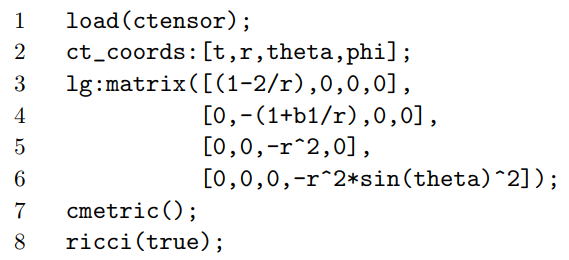
I won’t reproduce the entire output of the Ricci tensor, which is voluminous. We want all four of its nonvanishing components to vanish as quickly as possible for large values of r, so I decided to fiddle with Rtt, which looked as simple as any of them. It appears to vary as r−4 for large r, so let’s evaluate \(\lim_{r \rightarrow \infty} (r^{4} R_{tt})\):
The result is \(\dfrac{(b_{1}−2)}{2}\), so let’s set b1 = 2. The approximate solution we’ve found so far (reinserting the m’s),
\[ds^{2} \approx \left(1 - \dfrac{2m}{r}\right) dt^{2} - \left(1 + \dfrac{2m}{r}\right) dr^{2} - r^{2} d \theta^{2} - r^{2} \sin^{2} \theta d \phi^{2},\]
was first derived by Einstein in 1915, and he used it to solve the problem of the non-Keplerian relativistic correction to the orbit of Mercury, which was one of the first empirical tests of general relativity.
Continuing in this fashion, the results are as follows:
| $$\begin{split} a_{0} &= 1 \\ a_{1} &= -2 \\ a_{2} &= 0 \\ a_{3} &= 0 \end{split}$$ | $$\begin{split} b_{0} &= 1 \\ b_{1} &= 2 \\ b_{2} &= 4 \\ b_{2} &= 8 \end{split}$$ |
The Closed-form Solution
The solution is unexpectedly simple, and can be put into closed form. The approximate result we found for h was in fact exact. For k we have a geometric series \(\dfrac{1}{(1 − \dfrac{2}{r})}\), and when we reinsert the factor of m in the only way that makes the units work, we get \(\dfrac{1}{(1 − \dfrac{2m}{r})}\). The result for the metric is
\[ds^{2} = \left(1 - \dfrac{2m}{r}\right) dt^{2} - \left(\dfrac{1}{1 - \dfrac{2m}{r}}\right) dr^{2} - r^{2} d \theta^{2} - r^{2} \sin^{2} \theta d \phi^{2} \ldotp\]
This is called the Schwarzschild metric. A quick calculation in Maxima demonstrates that it is an exact solution for all r, i.e., the Ricci tensor vanishes everywhere, even at r < 2m, which is outside the radius of convergence of the geometric series.
Time-reversal Symmetry
The Schwarzschild metric is invariant under time reversal, since time occurs only in the form of \(dt^2\), which stays the same under dt → − dt. This is the same time-reversal symmetry that occurs in Newtonian gravity, where the field is described by the gravitational acceleration g, and accelerations are time-reversal invariant.
Fundamentally, this is an example of general relativity’s coordinate independence. The laws of physics provided by general relativity, such as the vacuum field equation, are invariant under any smooth coordinate transformation, and t → −t is such a coordinate transformation, so general relativity has time-reversal symmetry. Since the Schwarzschild metric was found by imposing time-reversalsymmetric boundary conditions on a time-reversal-symmetric differential equation, it is an equally valid solution when we time-reverse it. Furthermore, we expect the metric to be invariant under time reversal, unless spontaneous symmetry breaking occurs (see section 8.2).
This suggests that we ask the more fundamental question of what global symmetries general relativity has. Does it have symmetry under parity inversion, for example? Or can we take any solution such as the Schwarzschild spacetime and transform it into a frame of reference in which the source of the field is moving uniformly in a certain direction? Because general relativity is locally equivalent to special relativity, we know that these symmetries are locally valid. But it may not even be possible to define the corresponding global symmetries. For example, there are some spacetimes on which it is not even possible to define a global time coordinate. On such a spacetime, which is described as not time-orientable, there does not exist any smooth vector field that is everywhere timelike, so it is not possible to define past versus future light-cones at all points in space without having a discontinuous change in the definition occur somewhere. This is similar to the way in which a Möbius strip does not allow an orientation of its surface (an “up” direction as seen by an ant) to be defined globally.
Suppose that our spacetime is time-orientable, and we are able to define coordinates (p, q, r, s) such that p is always the timelike coordinate. Because q → −q is a smooth coordinate transformation, we are guaranteed that our spacetime remains a valid solution of the field equations under this change. But that doesn’t mean that what we’ve found is a symmetry under parity inversion in a plane. Our coordinate q is not necessarily interpretable as distance along a particular “q axis.” Such axes don’t even exist globally in general relativity. A coordinate does not even have to have units of time or distance; it could be an angle, for example, or it might not have any geometrical significance at all. Similarly, we could do a transformation q → q' = q + kp. If we think of q as measuring spatial position and p time, then this looks like a Galilean transformation, with k being the velocity. The solution to the field equations obtained after performing this transformation is still a valid solution, but that doesn’t mean that relativity has Galilean symmetry rather than Lorentz symmetry. There is no sensible way to define a Galilean transformation acting on an entire spacetime, because when we talk about a Galilean transformation we assume the existence of things like global coordinate axes, which do not even exist in general relativity.
References
3 “On the gravitational field of a point mass according to Einstein’s theory,” Sitzungsberichte der Koniglich Preussischen Akademie der Wissenschaften 1 (1916) 189. An English translation is available at http://arxiv.org/abs/physics/9905030v1.