
9.4: The Covariant Derivative
- Page ID
- 3476

\( \newcommand{\vecs}[1]{\overset { \scriptstyle \rightharpoonup} {\mathbf{#1}} } \)
\( \newcommand{\vecd}[1]{\overset{-\!-\!\rightharpoonup}{\vphantom{a}\smash {#1}}} \)
\( \newcommand{\dsum}{\displaystyle\sum\limits} \)
\( \newcommand{\dint}{\displaystyle\int\limits} \)
\( \newcommand{\dlim}{\displaystyle\lim\limits} \)
\( \newcommand{\id}{\mathrm{id}}\) \( \newcommand{\Span}{\mathrm{span}}\)
( \newcommand{\kernel}{\mathrm{null}\,}\) \( \newcommand{\range}{\mathrm{range}\,}\)
\( \newcommand{\RealPart}{\mathrm{Re}}\) \( \newcommand{\ImaginaryPart}{\mathrm{Im}}\)
\( \newcommand{\Argument}{\mathrm{Arg}}\) \( \newcommand{\norm}[1]{\| #1 \|}\)
\( \newcommand{\inner}[2]{\langle #1, #2 \rangle}\)
\( \newcommand{\Span}{\mathrm{span}}\)
\( \newcommand{\id}{\mathrm{id}}\)
\( \newcommand{\Span}{\mathrm{span}}\)
\( \newcommand{\kernel}{\mathrm{null}\,}\)
\( \newcommand{\range}{\mathrm{range}\,}\)
\( \newcommand{\RealPart}{\mathrm{Re}}\)
\( \newcommand{\ImaginaryPart}{\mathrm{Im}}\)
\( \newcommand{\Argument}{\mathrm{Arg}}\)
\( \newcommand{\norm}[1]{\| #1 \|}\)
\( \newcommand{\inner}[2]{\langle #1, #2 \rangle}\)
\( \newcommand{\Span}{\mathrm{span}}\) \( \newcommand{\AA}{\unicode[.8,0]{x212B}}\)
\( \newcommand{\vectorA}[1]{\vec{#1}} % arrow\)
\( \newcommand{\vectorAt}[1]{\vec{\text{#1}}} % arrow\)
\( \newcommand{\vectorB}[1]{\overset { \scriptstyle \rightharpoonup} {\mathbf{#1}} } \)
\( \newcommand{\vectorC}[1]{\textbf{#1}} \)
\( \newcommand{\vectorD}[1]{\overrightarrow{#1}} \)
\( \newcommand{\vectorDt}[1]{\overrightarrow{\text{#1}}} \)
\( \newcommand{\vectE}[1]{\overset{-\!-\!\rightharpoonup}{\vphantom{a}\smash{\mathbf {#1}}}} \)
\( \newcommand{\vecs}[1]{\overset { \scriptstyle \rightharpoonup} {\mathbf{#1}} } \)
\(\newcommand{\longvect}{\overrightarrow}\)
\( \newcommand{\vecd}[1]{\overset{-\!-\!\rightharpoonup}{\vphantom{a}\smash {#1}}} \)
\(\newcommand{\avec}{\mathbf a}\) \(\newcommand{\bvec}{\mathbf b}\) \(\newcommand{\cvec}{\mathbf c}\) \(\newcommand{\dvec}{\mathbf d}\) \(\newcommand{\dtil}{\widetilde{\mathbf d}}\) \(\newcommand{\evec}{\mathbf e}\) \(\newcommand{\fvec}{\mathbf f}\) \(\newcommand{\nvec}{\mathbf n}\) \(\newcommand{\pvec}{\mathbf p}\) \(\newcommand{\qvec}{\mathbf q}\) \(\newcommand{\svec}{\mathbf s}\) \(\newcommand{\tvec}{\mathbf t}\) \(\newcommand{\uvec}{\mathbf u}\) \(\newcommand{\vvec}{\mathbf v}\) \(\newcommand{\wvec}{\mathbf w}\) \(\newcommand{\xvec}{\mathbf x}\) \(\newcommand{\yvec}{\mathbf y}\) \(\newcommand{\zvec}{\mathbf z}\) \(\newcommand{\rvec}{\mathbf r}\) \(\newcommand{\mvec}{\mathbf m}\) \(\newcommand{\zerovec}{\mathbf 0}\) \(\newcommand{\onevec}{\mathbf 1}\) \(\newcommand{\real}{\mathbb R}\) \(\newcommand{\twovec}[2]{\left[\begin{array}{r}#1 \\ #2 \end{array}\right]}\) \(\newcommand{\ctwovec}[2]{\left[\begin{array}{c}#1 \\ #2 \end{array}\right]}\) \(\newcommand{\threevec}[3]{\left[\begin{array}{r}#1 \\ #2 \\ #3 \end{array}\right]}\) \(\newcommand{\cthreevec}[3]{\left[\begin{array}{c}#1 \\ #2 \\ #3 \end{array}\right]}\) \(\newcommand{\fourvec}[4]{\left[\begin{array}{r}#1 \\ #2 \\ #3 \\ #4 \end{array}\right]}\) \(\newcommand{\cfourvec}[4]{\left[\begin{array}{c}#1 \\ #2 \\ #3 \\ #4 \end{array}\right]}\) \(\newcommand{\fivevec}[5]{\left[\begin{array}{r}#1 \\ #2 \\ #3 \\ #4 \\ #5 \\ \end{array}\right]}\) \(\newcommand{\cfivevec}[5]{\left[\begin{array}{c}#1 \\ #2 \\ #3 \\ #4 \\ #5 \\ \end{array}\right]}\) \(\newcommand{\mattwo}[4]{\left[\begin{array}{rr}#1 \amp #2 \\ #3 \amp #4 \\ \end{array}\right]}\) \(\newcommand{\laspan}[1]{\text{Span}\{#1\}}\) \(\newcommand{\bcal}{\cal B}\) \(\newcommand{\ccal}{\cal C}\) \(\newcommand{\scal}{\cal S}\) \(\newcommand{\wcal}{\cal W}\) \(\newcommand{\ecal}{\cal E}\) \(\newcommand{\coords}[2]{\left\{#1\right\}_{#2}}\) \(\newcommand{\gray}[1]{\color{gray}{#1}}\) \(\newcommand{\lgray}[1]{\color{lightgray}{#1}}\) \(\newcommand{\rank}{\operatorname{rank}}\) \(\newcommand{\row}{\text{Row}}\) \(\newcommand{\col}{\text{Col}}\) \(\renewcommand{\row}{\text{Row}}\) \(\newcommand{\nul}{\text{Nul}}\) \(\newcommand{\var}{\text{Var}}\) \(\newcommand{\corr}{\text{corr}}\) \(\newcommand{\len}[1]{\left|#1\right|}\) \(\newcommand{\bbar}{\overline{\bvec}}\) \(\newcommand{\bhat}{\widehat{\bvec}}\) \(\newcommand{\bperp}{\bvec^\perp}\) \(\newcommand{\xhat}{\widehat{\xvec}}\) \(\newcommand{\vhat}{\widehat{\vvec}}\) \(\newcommand{\uhat}{\widehat{\uvec}}\) \(\newcommand{\what}{\widehat{\wvec}}\) \(\newcommand{\Sighat}{\widehat{\Sigma}}\) \(\newcommand{\lt}{<}\) \(\newcommand{\gt}{>}\) \(\newcommand{\amp}{&}\) \(\definecolor{fillinmathshade}{gray}{0.9}\)Learning Objectives
- A constant vector function, or for any tensor of higher rank changes when expressed in a new coordinate system
In this optional section we deal with the issues raised in section 7.5. We noted there that in non-Minkowski coordinates, one cannot naively use changes in the components of a vector as a measure of a change in the vector itself. A constant scalar function remains constant when expressed in a new coordinate system, but the same is not true for a constant vector function, or for any tensor of higher rank. This is because the change of coordinates changes the units in which the vector is measured, and if the change of coordinates is nonlinear, the units vary from point to point. This topic doesn’t logically belong in this chapter, but I’ve placed it here because it can’t be discussed clearly without already having covered tensors of rank higher than one.
Consider the one-dimensional case, in which a vector \(v^a\) has only one component, and the metric is also a single number, so that we can omit the indices and simply write \(v\) and \(g\). (We just have to remember that \(v\) is really a vector, even though we’re leaving out the upper index.) If \(v\) is constant, its derivative \(dv/ dx\), computed in the ordinary way without any correction term, is zero. If we further assume that the metric is simply the constant \(g = 1\), then zero is not just the answer but the right answer.
Now suppose we transform into a new coordinate system \(X\), and the metric \(G\), expressed in this coordinate system, is not constant. Applying the tensor transformation law, we have \(V = v\frac{\mathrm{d} X}{\mathrm{d} x}\), and differentiation with respect to \(X\) will not give zero, because the factor \(dX/ dx\) isn’t constant. This is the wrong answer: \(V\) isn’t really varying, it just appears to vary because \(G\) does.
We want to add a correction term onto the derivative operator \(d/ dX\), forming a new derivative operator \(∇_X\) that gives the right answer. \(∇_X\) is called the covariant derivative. This correction term is easy to find if we consider what the result ought to be when differentiating the metric itself. In general, if a tensor appears to vary, it could vary either because it really does vary or because the metric varies. If the metric itself varies, it could be either because the metric really does vary or . . . because the metric varies. In other words, there is no sensible way to assign a nonzero covariant derivative to the metric itself, so we must have \(∇_X G = 0\). The required correction therefore consists of replacing \(d/ dX\) with
\[\nabla _X = \frac{\mathrm{d} }{\mathrm{d} X} - G^{-1}\frac{\mathrm{d} G}{\mathrm{d} X}\]
Applying this to \(G\) gives zero. \(G\) is a second-rank tensor with two lower indices. If we apply the same correction to the derivatives of other tensors of this type, we will get nonzero results, and they will be the right nonzero results. Mathematically, the form of the derivative is \(\frac{1}{y}\; \frac{\mathrm{d} y}{\mathrm{d} x}\), which is known as a logarithmic derivative, since it equals \(\frac{\mathrm{d} (\ln y)}{\mathrm{d} x}\). It measures the multiplicative rate of change of \(y\). For example, if \(y\) scales up by a factor of \(k\) when \(x\) increases by \(1\) unit, then the logarithmic derivative of \(y\) is \(\ln k\). The logarithmic derivative of \(e^{cx}\) is \(c\). The logarithmic nature of the correction term to \(∇_X\) is a good thing, because it lets us take changes of scale, which are multiplicative changes, and convert them to additive corrections to the derivative operator. The additivity of the corrections is necessary if the result of a covariant derivative is to be a tensor, since tensors are additive creatures. What about quantities that are not second-rank covariant tensors? Under a rescaling of coordinates by a factor of \(k\), covectors scale by \(k^{-1}\), and second-rank tensors with two lower indices scale by \(k^{-2}\). The correction term should therefore be half as much for covectors,
\[\nabla _X = \frac{\mathrm{d} }{\mathrm{d} X} - \frac{1}{2}G^{-1}\frac{\mathrm{d} G}{\mathrm{d} X}\]
and should have an opposite sign for vectors.
Generalizing the correction term to derivatives of vectors in more than one dimension, we should have something of this form:
\[\nabla _a v^b = \partial _a v^b + \Gamma ^b\: _{ac} v^c\]
\[\nabla _a v^b = \partial _a v^b - \Gamma ^c\: _{ba} v_c\]
where \(Γ^b\: _{ac}\), called the Christoffel symbol, does not transform like a tensor, and involves derivatives of the metric. (“Christoffel” is pronounced “Krist-AWful,” with the accent on the middle syllable.)
An important gotcha is that when we evaluate a particular component of a covariant derivative such as \(∇_2 v^3\), it is possible for the result to be nonzero even if the component \(v^3\) vanishes identically.
Example \(\PageIndex{1}\): Christoffel symbols on the globe
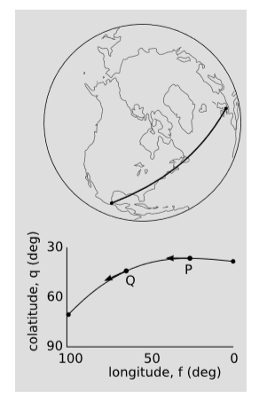
As a qualitative example, consider the airplane trajectory shown in figure \(\PageIndex{2}\), from London to Mexico City. This trajectory is the shortest one between these two points; such a minimum-length trajectory is called a geodesic. In physics it is customary to work with the colatitude, \(θ\), measured down from the north pole, rather then the latitude, measured from the equator. At \(P\), over the North Atlantic, the plane’s colatitude has a minimum. (We can see, without having to take it on faith from the figure, that such a minimum must occur. The easiest way to convince oneself of this is to consider a path that goes directly over the pole, at \(θ = 0\).)
At \(P\), the plane’s velocity vector points directly west. At \(Q\), over New England, its velocity has a large component to the south. Since the path is a geodesic and the plane has constant speed, the velocity vector is simply being parallel-transported; the vector’s covariant derivative is zero. Since we have \(v_θ = 0\) at \(P\), the only way to explain the nonzero and positive value of \(∂_φ v^θ\) is that we have a nonzero and negative value of \(Γ^θ\: _{φφ}\).
By symmetry, we can infer that \(Γ^θ\: _{φφ}\) must have a positive value in the southern hemisphere, and must vanish at the equator.
\(Γ^θ\:_{φφ}\) is computed in example below.
Symmetry also requires that this Christoffel symbol be independent of \(φ\), and it must also be independent of the radius of the sphere.
To compute the covariant derivative of a higher-rank tensor, we just add more correction terms, e.g.,
\[\nabla _a U_{bc} = \partial _a U_{bc} - \Gamma ^d\: _{ba}U_{dc} - \Gamma ^d\: _{ca}U_{bd}\]
or
\[\nabla _a U_{b}^c = \partial _a U_{b}^c - \Gamma ^d\: _{ba}U_{d}^c - \Gamma ^c\: _{ad}U_{b}^d\]
With the partial derivative \(∂_µ\), it does not make sense to use the metric to raise the index and form \(∂_µ\). It does make sense to do so with covariant derivatives, so \(\nabla ^a = g^{ab} \nabla _b\) is a correct identity.
Comma, semicolon, and birdtracks notation
Some authors use superscripts with commas and semicolons to indicate partial and covariant derivatives. The following equations give equivalent notations for the same derivatives:
\[\partial _\mu = \frac{\partial }{\partial x^\mu }\]
\[\partial _\mu X_\nu = X_{\nu ,\mu }\]
\[\nabla _a X_b = X_{b;a}\]
\[\nabla ^a X_b = X_b\: ^{;a}\]
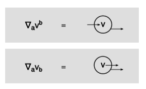
Figure \(\PageIndex{3}\) shows two examples of the corresponding birdtracks notation. Because birdtracks are meant to be manifestly coordinateindependent, they do not have a way of expressing non-covariant derivatives.
Finding the Christoffel symbol from the metric
We’ve already found the Christoffel symbol in terms of the metric in one dimension. Expressing it in tensor notation, we have
\[\Gamma ^d\: _{ba} = \frac{1}{2}g^{cd}(\partial _? g_{??})\]
where inversion of the one-component matrix \(G\) has been replaced by matrix inversion, and, more importantly, the question marks indicate that there would be more than one way to place the subscripts so that the result would be a grammatical tensor equation. The most general form for the Christoffel symbol would be
\[\Gamma ^b\: _{ac} = \frac{1}{2}g^{db}(L\partial _c g_{ab} + M\partial _a g_{cb} + N\partial _b g_{ca})\]
where \(L\), \(M\), and \(N\) are constants. Consistency with the one dimensional expression requires \(L + M + N = 1\). The condition \(L = M\) arises on physical, not mathematical grounds; it reflects the fact that experiments have not shown evidence for an effect called torsion, in which vectors would rotate in a certain way when transported. The \(L\) and \(M\) terms have a different physical significance than the \(N\) term.
Suppose an observer uses coordinates such that all objects are described as lengthening over time, and the change of scale accumulated over one day is a factor of \(k > 1\). This is described by the derivative \(∂_t g_{xx} < 1\), which affects the \(M\) term. Since the metric is used to calculate squared distances, the \(g_{xx}\) matrix element scales down by \(1/√k\). To compensate for \(∂_t v^x < 0\), so we need to add a positive correction term, \(M > 0\), to the covariant derivative. When the same observer measures the rate of change of a vector \(v^t\) with respect to space, the rate of change comes out to be too small, because the variable she differentiates with respect to is too big. This requires \(N < 0\), and the correction is of the same size as the \(M\) correction, so \(|M| = |N|\). We find \(L = M = -N = 1\).
Self-check: Does the above argument depend on the use of space for one coordinate and time for the other?
The resulting general expression for the Christoffel symbol in terms of the metric is
\[\Gamma ^c\: _{ab} = \frac{1}{2}g^{cd}(\partial _a g_{bd} + \partial _b g_{ad} - \partial _d g_{ab})\]
One can go back and check that this gives \(\nabla _c g_{ab} = 0\).
Self-check: In the case of \(1\) dimension, show that this reduces to the earlier result of \(-\frac{1}{2}\frac{\mathrm{d} G}{\mathrm{d} X}\).
\(Γ\) is not a tensor, i.e., it doesn’t transform according to the tensor transformation rules. Since \(Γ\) isn’t a tensor, it isn’t obvious that the covariant derivative, which is constructed from it, is tensorial. But if it isn’t obvious, neither is it surprising – the goal of the above derivation was to get results that would be coordinate-independent.
Example \(\PageIndex{2}\): Christoffel symbols on the globe, quantitatively
In Example \(\PageIndex{1}\), we inferred the following properties for the Christoffel symbol \(Γ^θ\: _{φφ}\) on a sphere of radius \(R: Γ^θ\: _{φφ}\) is independent of \(φ\) and \(R\), \(Γ^θ\: _{φφ} < 0\) in the northern hemisphere (colatitude \(θ\) less than \(π/2\)), \(Γ^θ\: _{φφ} = 0\) on the equator, and \(Γ^θ\: _{φφ} > 0\) in the southern hemisphere.
The metric on a sphere is \(ds^2 = R^2 dθ^2 + R^2 sin^2 θdφ^2\). The only nonvanishing term in the expression for \(Γ^θ\: _{φφ}\) is the one involving \(∂_θ g_{φφ} = 2R^2 sinθcosθ\). The result is \(Γ^θ\: _{φφ} = -sinθcosθ\), which can be verified to have the properties claimed above.
The geodesic equation
A world-line is a timelike curve in spacetime. As a special case, some such curves are actually not curved but straight. Physically, the ones we consider straight are those that could be the worldline of a test particle not acted on by any non-gravitational forces (section 5.1). Mathematically, we will show in this section how the Christoffel symbols can be used to find differential equations that describe such motion. The world-line of a test particle is called a geodesic. The equations also have solutions that are spacelike or lightlike, and we consider these to be geodesics as well.
Geodesics play the same role in relativity that straight lines play in Euclidean geometry. In Euclidean geometry, we can specify two points and ask for the curve connecting them that has minimal length. The answer is a line. In special relativity, a timelike geodesic maximizes the proper time (section 2.4) between two events.
In special relativity, geodesics are given by linear equations when expressed in Minkowski coordinates, and the velocity vector of a test particle has constant components when expressed in Minkowski coordinates. In general relativity, Minkowski coordinates don’t exist, and geodesics don’t have the properties we expect based on Euclidean intuition; for example, initially parallel geodesics may later converge or diverge.
Characterization of the geodesic
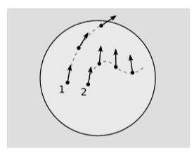
A geodesic can be defined as a world-line that preserves tangency under parallel transport, figure \(\PageIndex{4}\). This is essentially a mathematical way of expressing the notion that we have previously expressed more informally in terms of “staying on course” or moving “inertially.” (For reasons discussed in more detail below, this definition is preferable to defining a geodesic as a curve of extremal or stationary metric length.)
A curve can be specified by giving functions \(x^i(λ)\) for its coordinates, where \(λ\) is a real parameter. A vector lying tangent to the curve can then be calculated using partial derivatives, \(T^i = ∂x^i/∂λ\). There are three ways in which a vector function of \(λ\) could change:
- it could change for the trivial reason that the metric is changing, so that its components changed when expressed in the new metric
- it could change its components perpendicular to the curve; or
- it could change its component parallel to the curve.
Possibility 1 should not really be considered a change at all, and the definition of the covariant derivative is specifically designed to be insensitive to this kind of thing. 2 cannot apply to \(T^i\), which is tangent by construction. It would therefore be convenient if \(T^i\) happened to be always the same length. If so, then 3 would not happen either, and we could reexpress the definition of a geodesic by saying that the covariant derivative of \(T^i\) was zero. For this reason, we will assume for the remainder of this section that the parametrization of the curve has this property. In a Newtonian context, we could imagine the \(x^i\) to be purely spatial coordinates, and \(λ\) to be a universal time coordinate. We would then interpret \(T^i\) as the velocity, and the restriction would be to a parametrization describing motion with constant speed. In relativity, the restriction is that \(λ\) must be an affine parameter. For example, it could be the proper time of a particle, if the curve in question is timelike.
Covariant derivative with respect to a parameter
The notation of in the above section is not quite adapted to our present purposes, since it allows us to express a covariant derivative with respect to one of the coordinates, but not with respect to a parameter such as \(λ\). We would like to notate the covariant derivative of \(T^i\) with respect to \(λ\) as \(∇_λ T^i\), even though \(λ\) isn’t a coordinate. To connect the two types of derivatives, we can use a total derivative. To make the idea clear, here is how we calculate a total derivative for a scalar function \(f(x,y)\), without tensor notation:
\[\frac{\mathrm{d} f}{\mathrm{d} \lambda } = \frac{\partial f}{\partial x} \frac{\partial x}{\partial \lambda } + \frac{\partial f}{\partial y} \frac{\partial y}{\partial \lambda }\]
This is just the generalization of the chain rule to a function of two variables. For example, if \(λ\) represents time and \(f\) temperature, then this would tell us the rate of change of the temperature as a thermometer was carried through space. Applying this to the present problem, we express the total covariant derivative as
\[\begin{align*} \nabla _{\lambda } T^i &= (\nabla _b T^i)\frac{\mathrm{d} x^b}{\mathrm{d} \lambda }\\ &= (\partial _b T^i + \Gamma ^i \: _{bc}T^c)\frac{\mathrm{d} x^b}{\mathrm{d} \lambda } \end{align*}\]
The geodesic equation
Recognizing \(\partial _b T^i \frac{\mathrm{d} x^b}{\mathrm{d} \lambda }\) as a total non-covariant derivative, we find
\[\nabla _{\lambda } T^i = \frac{\mathrm{d} T^i}{\mathrm{d} \lambda } + \Gamma ^i\: _{bc} T^c \frac{\mathrm{d} x^b}{\mathrm{d} \lambda }\]
Substituting \(\frac{\partial x^i}{\partial\lambda }\) for \(T^i\), and setting the covariant derivative equal to zero, we obtain
\[\frac{\mathrm{d}^2 x^i}{\mathrm{d} \lambda ^2} + \Gamma ^i\: _{bc} \frac{\mathrm{d} x^c}{\mathrm{d} \lambda }\frac{\mathrm{d} x^b}{\mathrm{d} \lambda } = 0\]
This is known as the geodesic equation.
If this differential equation is satisfied for one affine parameter \(λ\), then it is also satisfied for any other affine parameter \(λ' = aλ + b\), where \(a\) and \(b\) are constants. Recall that affine parameters are only defined along geodesics, not along arbitrary curves. We can’t start by defining an affine parameter and then use it to find geodesics using this equation, because we can’t define an affine parameter without first specifying a geodesic. Likewise, we can’t do the geodesic first and then the affine parameter, because if we already had a geodesic in hand, we wouldn’t need the differential equation in order to find a geodesic. The solution to this chicken-and-egg conundrum is to write down the differential equations and try to find a solution, without trying to specify either the affine parameter or the geodesic in advance.
The geodesic equation is useful in establishing one of the necessary theoretical foundations of relativity, which is the uniqueness of geodesics for a given set of initial conditions. If the geodesic were not uniquely determined, then particles would have no way of deciding how to move. The form of the geodesic equation guarantees uniqueness, because one can use it to define an algorithm that constructs a geodesic for a given set of initial conditions.
Not characterizable as curves of stationary length
The geodesic equation may seem cumbersome. Why not just define a geodesic as a curve connecting two points that maximizes or minimizes its own metric length? The trouble is that this doesn’t generalize nicely to curves that are not timelike. The casual reader may wish to skip the remainder of this subsection, which discusses this point.
For the spacelike case, we would want to define the proper metric length \(σ\) of a curve as \(\sigma = \int \sqrt{-g{ij} dx^i dx^j}\), the minus sign being necessary because we are using a metric with signature \(+---\), and we want the result to be real. The quantity \(σ\) can be thought of as the result we would get by approximating the curve with a chain of short line segments, and adding their proper lengths. In the case where the whole curve lies within a plane of simultaneity for some observer, \(σ\) is the curve’s Euclidean length as measured by that observer. Our \(σ\) is neither a maximum nor a minimum for a spacelike geodesic connecting two events. To see this, pick a frame in which the two events are simultaneous, and adopt Minkowski coordinates such that the points both lie on the \(x\)-axis. Deforming the geodesic in the \(xy\) plane does what we expect according to Euclidean geometry: it increases the length. Deforming it in the \(xt\) plane, however, reduces the length (as becomes obvious when you consider the case of a large deformation that turns the geodesic into a curve of length zero, consisting of two lightlike line segments). The result is that the geodesic is neither a minimizer nor a maximizer of \(σ\).
Maximizing or minimizing the proper length is a strong requirement. A related but more permissive criterion to apply to a curve connecting two fixed points is that if we vary the curve by some small amount, the variation in length should vanish to first order. For example, two points \(A\) and \(B\) on the surface of the earth determine a great circle, i.e., a circle whose circumference equals that of the earth. This great circle gives us two different paths by which we could travel from \(A\) to \(B\). One of these will usually be longer than the other. Both of these are as straight as they can be while keeping to the surface of the earth, so in this context of spherical geometry they are both considered to be geodesics. One thing that the two paths have in common is that they are both stationary. Stationarity is defined as follows. Given a certain parametrized curve \(γ(t)\), let us fix some vector \(h(t)\) at each point on the curve that is tangent to the earth’s surface, and let \(h\) be a continuous function of \(t\) that vanishes at the end-points. Then if is small compared to the radius of the earth, we can clearly define what it means to perturb \(γ\) by \(h\), producing another curve \(γ∗\) similar to, but not the same as, \(γ\). Stationarity means that the difference in length between \(γ\) and \(γ∗\) is of order \(2\) for small . This is a generalization of the elementary calculus notion that a function has a zero derivative near an extremum or point of inflection. In our example on the surface of the earth, the two geodesics connecting \(A\) and \(B\) are both stationary.
Spacelike geodesics in special relativity are stationary by the above definition. However, this assertion may be misleading. Because we construct the displacement as the product \(h\), its derivative is also guaranteed to shrink in proportion to for small . We could loosen this requirement a little bit, and only require that the magnitude of the displacement be of order . In this case, one can show that spacelike curves are not stationary. For example, any spacelike curve can be approximated to an arbitrary degree of precision by a chain of lightlike geodesic segments. Thus an arbitrarily small perturbation in the curve reduces its length to zero.
The situation becomes even worse for lightlike geodesics. Here we would have to define what “length” was. We could either take an absolute value, \(L = \int \sqrt{|g{ij} dx^i dx^j|}\), or not, \(L = \int \sqrt{g{ij} dx^i dx^j}\). If we don’t take the absolute value, \(L\) need not be real for small variations of the geodesic, and therefore we don’t have a well-defined ordering, and can’t say whether \(L\) is a maximum, a minimum, or neither. Regardless of whether we take the absolute value, we have \(L = 0\) for a lightlike geodesic, but the square root function doesn’t have differentiable behavior when its argument is zero, so we don’t have stationarity. If we do take the absolute value, then for the geodesic curve, the length is zero, which is the shortest possible. However, one can have nongeodesic curves of zero length, such as a lightlike helical curve about the \(t\)-axis.