17.9: Viscosity and Turbulence

Learning Objectives

• Explain what viscosity is
• Calculate flow and resistance with Poiseuille's law
• Explain how pressure drops due to resistance
• Calculate the Reynolds number for an object moving through a fluid
• Use the Reynolds number for a system to determine whether it is laminar or turbulent
• Describe the conditions under which an object has a terminal speed

In Applications of Newton’s Laws, which introduced the concept of friction, we saw that an object sliding across the floor with an initial velocity and no applied force comes to rest due to the force of friction. Friction depends on the types of materials in contact and is proportional to the normal force. We also discussed drag and air resistance in that same chapter. We explained that at low speeds, the drag is proportional to the velocity, whereas at high speeds, drag is proportional to the velocity squared. In this section, we introduce the forces of friction that act on fluids in motion. For example, a fluid flowing through a pipe is subject to resistance, a type of friction, between the fluid and the walls. Friction also occurs between the different layers of fluid. These resistive forces affect the way the fluid flows through the pipe.

Viscosity and Laminar Flow

When you pour yourself a glass of juice, the liquid flows freely and quickly. But if you pour maple syrup on your pancakes, that liquid flows slowly and sticks to the pitcher. The difference is fluid friction, both within the fluid itself and between the fluid and its surroundings. We call this property of fluids viscosity. Juice has low viscosity, whereas syrup has high viscosity.

The precise definition of viscosity is based on laminar, or nonturbulent, flow. Figure $\PageIndex{1}$ shows schematically how laminar and turbulent flow differ. When flow is laminar, layers flow without mixing. When flow is turbulent, the layers mix, and significant velocities occur in directions other than the overall direction of flow.

Figure $\PageIndex{1}$: (a) Laminar flow occurs in layers without mixing. Notice that viscosity causes drag between layers as well as with the fixed surface. The speed near the bottom of the flow (v_b) is less than speed near the top (v_t) because in this case, the surface of the containing vessel is at the bottom. (b) An obstruction in the vessel causes turbulent flow. Turbulent flow mixes the fluid. There is more interaction, greater heating, and more resistance than in laminar flow.

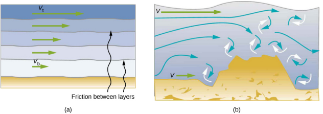
Turbulence is a fluid flow in which layers mix together via eddies and swirls. It has two main causes. First, any obstruction or sharp corner, such as in a faucet, creates turbulence by imparting velocities perpendicular to the flow. Second, high speeds cause turbulence. The drag between adjacent layers of fluid and between the fluid and its surroundings can form swirls and eddies if the speed is great enough. In Figure $\PageIndex{2}$, the speed of the accelerating smoke reaches the point that it begins to swirl due to the drag between the smoke and the surrounding air.

Figure $\PageIndex{2}$: Smoke rises smoothly for a while and then begins to form swirls and eddies. The smooth flow is called laminar flow, whereas the swirls and eddies typify turbulent flow. Smoke rises more rapidly when flowing smoothly than after it becomes turbulent, suggesting that turbulence poses more resistance to flow. (credit: “Creativity103”/Flickr)

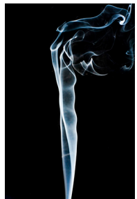
Figure $\PageIndex{3}$ shows how viscosity is measured for a fluid. The fluid to be measured is placed between two parallel plates. The bottom plate is held fixed, while the top plate is moved to the right, dragging fluid with it. The layer (or lamina) of fluid in contact with either plate does not move relative to the plate, so the top layer moves at speed v while the bottom layer remains at rest. Each successive layer from the top down exerts a force on the one below it, trying to drag it along, producing a continuous variation in speed from v to 0 as shown. Care is taken to ensure that the flow is laminar, that is, the layers do not mix. The motion in the figure is like a continuous shearing motion. Fluids have zero shear strength, but the rate at which they are sheared is related to the same geometrical factors A and L as is shear deformation for solids. In the diagram, the fluid is initially at rest. The layer of fluid in contact with the moving plate is accelerated and starts to move due to the internal friction between moving plate and the fluid. The next layer is in contact with the moving layer; since there is internal friction between the two layers, it also accelerates, and so on through the depth of the fluid. There is also internal friction between the stationary plate and the lowest layer of fluid, next to the station plate. The force is required to keep the plate moving at a constant velocity due to the internal friction.

Figure $\PageIndex{3}$: Measurement of viscosity for laminar flow of fluid between two plates of area A. The bottom plate is fixed. When the top plate is pushed to the right, it drags the fluid along with it.

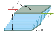
A force F is required to keep the top plate in Figure $\PageIndex{3}$ moving at a constant velocity v, and experiments have shown that this force depends on four factors. First, F is directly proportional to v (until the speed is so high that turbulence occurs—then a much larger force is needed, and it has a more complicated dependence on v). Second, F is proportional to the area A of the plate. This relationship seems reasonable, since A is directly proportional to the amount of fluid being moved. Third, F is inversely proportional to the distance between the plates L. This relationship is also reasonable; L is like a lever arm, and the greater the lever arm, the less the force that is needed. Fourth, F is directly proportional to the coefficient of viscosity, $\eta$ The greater the viscosity, the greater the force required. These dependencies are combined into the equation

$$F = \eta \frac{vA}{L} \ldotp$$

This equation gives us a working definition of fluid viscosity $\eta$. Solving for $\eta$ gives

$$\eta = \frac{FL}{vA} \label{14.17}$$

which defines viscosity in terms of how it is measured. The SI unit of viscosity is $\frac{N\; \cdotp m}{[(m/s)m^{2}]}$ = (N/m²)s or Pa • s. Table $\PageIndex{1}$ lists the coefficients of viscosity for various fluids. Viscosity varies from one fluid to another by several orders of magnitude. As you might expect, the viscosities of gases are much less than those of liquids, and these viscosities often depend on temperature.

Table $\PageIndex{1}$: Coefficients of Viscosity of Various Fluids

Fluid	Temperature (°C)	Viscosity $\eta \times 10^{3}$
Air	0	0.0171
	20	0.0181
	40	0.0190
	100	0.0218
Ammonia	20	0.00974
Carbon dioxide	20	0.0147
Helium	20	0.0196
Hydrogen	0	0.0090
Mercury	20	0.0450
Oxygen	20	0.0203
Steam	100	0.0130
Liquid water	0	1.792
	20	1.002
	37	0.6947
	40	0.653
	100	0.282
Whole blood	20	3.015
	37	2.084
Blood plasma	20	1.810
	37	1.257
Ethyl alcohol	20	1.20
Methanol	20	0.584
Oil (heavy machine)	20	660
Oil (motor, SAE 10)	30	200
Oil (olive)	20	138
Glycerin	20	1500
Honey	20	2000-10000
Maple syrup	20	2000-3000
Milk	20	3.0
Oil (corn)	20	65

Laminar Flow Confined to Tubes: Poiseuille’s Law

What causes flow? The answer, not surprisingly, is a pressure difference. In fact, there is a very simple relationship between horizontal flow and pressure. Flow rate $Q$ is in the direction from high to low pressure. The greater the pressure differential between two points, the greater the flow rate. This relationship can be stated as

$$Q = \frac{p_{2} - p_{1}}{R}$$

where $p_1$ and $p_2$ are the pressures at two points, such as at either end of a tube, and $R$ is the resistance to flow. The resistance $R$ includes everything, except pressure, that affects flow rate. For example, $R$ is greater for a long tube than for a short one. The greater the viscosity of a fluid, the greater the value of $R$. Turbulence greatly increases R, whereas increasing the diameter of a tube decreases $R$.

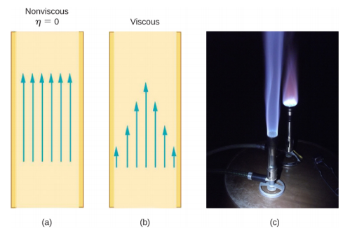
If viscosity is zero, the fluid is frictionless and the resistance to flow is also zero. Comparing frictionless flow in a tube to viscous flow, as in Figure $\PageIndex{4}$, we see that for a viscous fluid, speed is greatest at midstream because of drag at the boundaries. We can see the effect of viscosity in a Bunsen burner flame [part (c)], even though the viscosity of natural gas is small.

Figure $\PageIndex{4}$: (a) If fluid flow in a tube has negligible resistance, the speed is the same all across the tube. (b) When a viscous fluid flows through a tube, its speed at the walls is zero, increasing steadily to its maximum at the center of the tube. (c) The shape of a Bunsen burner flame is due to the velocity profile across the tube. (credit c: modification of work by Jason Woodhead)

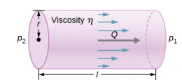
The resistance R to laminar flow of an incompressible fluid with viscosity $\eta$ through a horizontal tube of uniform radius r and length l, is given by

$$R = \frac{8 \eta l}{\pi r^{4}} \ldotp \label{14.18}$$

This equation is called Poiseuille’s law for resistance, named after the French scientist J. L. Poiseuille (1799–1869), who derived it in an attempt to understand the flow of blood through the body.

Let us examine Poiseuille’s expression for R to see if it makes good intuitive sense. We see that resistance is directly proportional to both fluid viscosity $\eta$ and the length l of a tube. After all, both of these directly affect the amount of friction encountered—the greater either is, the greater the resistance and the smaller the flow. The radius r of a tube affects the resistance, which again makes sense, because the greater the radius, the greater the flow (all other factors remaining the same). But it is surprising that r is raised to the fourth power in Poiseuille’s law. This exponent means that any change in the radius of a tube has a very large effect on resistance. For example, doubling the radius of a tube decreases resistance by a factor of 2⁴ = 16.

Taken together $Q = \frac{p_{2} - p_{1}}{R}$ and $R = \frac{8 \eta l}{\pi r^{4}}$ give the following expression for flow rate:

$$Q = \frac{(p_{2} - p_{1}) \pi r^{4}}{8 \eta l} \ldotp \label{14.19}$$

This equation describes laminar flow through a tube. It is sometimes called Poiseuille’s law for laminar flow, or simply Poiseuille’s law (Figure $\PageIndex{5}$).

Figure $\PageIndex{5}$: Poiseuille’s law applies to laminar flow of an incompressible fluid of viscosity η through a tube of length l and radius r. The direction of flow is from greater to lower pressure. Flow rate Q is directly proportional to the pressure difference p₂ − p₁, and inversely proportional to the length l of the tube and viscosity $\eta$ of the fluid. Flow rate increases with radius by a factor of r⁴.

Example 14.8: Using Flow Rate - Air Conditioning Systems

An air conditioning system is being designed to supply air at a gauge pressure of 0.054 Pa at a temperature of 20 °C. The air is sent through an insulated, round conduit with a diameter of 18.00 cm. The conduit is 20-meters long and is open to a room at atmospheric pressure 101.30 kPa. The room has a length of 12 meters, a width of 6 meters, and a height of 3 meters. (a) What is the volume flow rate through the pipe, assuming laminar flow? (b) Estimate the length of time to completely replace the air in the room. (c) The builders decide to save money by using a conduit with a diameter of 9.00 cm. What is the new flow rate?

Strategy

Assuming laminar flow, Poiseuille’s law states that

$$Q = \frac{(p_{2} - p_{1}) \pi r^{4}}{8 \eta l} = \frac{dV}{dt} \ldotp \nonumber$$

We need to compare the artery radius before and after the flow rate reduction. Note that we are given the diameter of the conduit, so we must divide by two to get the radius.

Solution

1. Assuming a constant pressure difference and using the viscosity $\eta = 0.0181\; mPa\; \cdotp s$, $$Q = \frac{(0.054\; Pa)(3.14)(0.09\; m)^{4}}{8(0.0181 \times 10^{-3}\; Pa\; \cdotp s)(20\; m)} = 3.84 \times 10^{-3}\; m^{3}/s \ldotp$$
2. Assuming constant flow $Q = \frac{dV}{dt} \approx \frac{\Delta V}{\Delta t}$ $$\Delta t = \frac{\Delta V}{Q} = \frac{(12\; m)(6\; m)(3\; m)}{3.84 \times 10^{-3}\; m^{3}/s} = 5.63 \times 10^{4}\; s = 15.63\; hr \ldotp \nonumber$$
3. Using laminar flow, Poiseuille’s law yields $$Q = \frac{(0.054\; Pa)(3.14)(0.045\; m){4}}{8(0.0181 \times 10^{-3}\; Pa\; \cdotp s)(20\; m)} = 22.40 \times 10^{-4}\; m^{3}/s \ldotp$$ Thus, the radius of the conduit decreases by half reduces the flow rate to 6.25% of the original value.

Significance

In general, assuming laminar flow, decreasing the radius has a more dramatic effect than changing the length. If the length is increased and all other variables remain constant, the flow rate is decreased:

$$\begin{split} \frac{Q_{A}}{Q_{B}} & = \frac{\frac{(p_{2} - p_{1}) \pi r_{A}^{4}}{8 \eta l_{A}}}{\frac{(p_{2} - p_{1}) \pi r_{B}^{4}}{8 \eta l_{B}}} = \frac{l_{B}}{l_{A}} \\ Q_{B} & = \frac{l_{A}}{l_{B}} Q_{A} \ldotp \end{split} \nonumber$$

Doubling the length cuts the flow rate to one-half the original flow rate.

If the radius is decreased and all other variables remain constant, the volume flow rate decreases by a much larger factor.

$$\begin{split} \frac{Q_{A}}{Q_{B}} & = \frac{\frac{(p_{2} - p_{1}) \pi r_{A}^{4}}{8 \eta l_{A}}}{\frac{(p_{2} - p_{1}) \pi r_{B}^{4}}{8 \eta l_{B}}} = \left(\dfrac{r_{A}}{r_{B}}\right)^{4} \\ Q_{B} & = \left(\dfrac{r_{B}}{r_{A}}\right)^{4} Q_{A} \end{split}$$

Cutting the radius in half decreases the flow rate to one-sixteenth the original flow rate.

Flow and Resistance as Causes of Pressure Drops

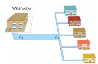
Water pressure in homes is sometimes lower than normal during times of heavy use, such as hot summer days. The drop in pressure occurs in the water main before it reaches individual homes. Let us consider flow through the water main as illustrated in Figure $\PageIndex{6}$. We can understand why the pressure p₁ to the home drops during times of heavy use by rearranging the equation for flow rate:

$$\begin{align} Q & = \frac{p_{2} - p_{1}}{R} \\[4pt] p_{2} - p_{1} & = RQ . \label{EQ5} \end{align}$$

In this case, $p_2$ is the pressure at the water works and $R$ is the resistance of the water main. During times of heavy use, the flow rate $Q$ is large. This means that $p_2 − p_1$ must also be large. Thus $p_1$ must decrease. It is correct to think of flow and resistance as causing the pressure to drop from p₂ to p₁. The equation p₂ − p₁ = RQ is valid for both laminar and turbulent flows.

Figure $\PageIndex{6}$: During times of heavy use, there is a significant pressure drop in a water main, and p₁ supplied to users is significantly less than p₂ created at the water works. If the flow is very small, then the pressure drop is negligible, and p₂ ≈ p₁.

We can also use Equation $\ref{EQ5}$ to analyze pressure drops occurring in more complex systems in which the tube radius is not the same everywhere. Resistance is much greater in narrow places, such as in an obstructed coronary artery. For a given flow rate Q, the pressure drop is greatest where the tube is most narrow. This is how water faucets control flow. Additionally, R is greatly increased by turbulence, and a constriction that creates turbulence greatly reduces the pressure downstream. Plaque in an artery reduces pressure and hence flow, both by its resistance and by the turbulence it creates.

Measuring Turbulence

An indicator called the Reynolds number $N_R$ can reveal whether flow is laminar or turbulent. For flow in a tube of uniform diameter, the Reynolds number is defined as

$$N_{R} = \frac{2 \rho vr}{\eta}\; (flow\; in\; tube) \label{14.20}$$

where $\rho$ is the fluid density, v its speed, $\eta$ its viscosity, and $r$ the tube radius. The Reynolds number is a dimensionless quantity. Experiments have revealed that $N_R$ is related to the onset of turbulence. For N_R below about 2000, flow is laminar. For $N_R$ above about 3000, flow is turbulent.

For values of $N_R$ between about 2000 and 3000, flow is unstable—that is, it can be laminar, but small obstructions and surface roughness can make it turbulent, and it may oscillate randomly between being laminar and turbulent. In fact, the flow of a fluid with a Reynolds number between 2000 and 3000 is a good example of chaotic behavior. A system is defined to be chaotic when its behavior is so sensitive to some factor that it is extremely difficult to predict. It is difficult, but not impossible, to predict whether flow is turbulent or not when a fluid’s Reynold’s number falls in this range due to extremely sensitive dependence on factors like roughness and obstructions on the nature of the flow. A tiny variation in one factor has an exaggerated (or nonlinear) effect on the flow.

Example 14.9: Using Flow Rate - Turbulent Flow or Laminar Flow

In Example 14.8, we found the volume flow rate of an air conditioning system to be Q = 3.84 x 10⁻³ m³/s. This calculation assumed laminar flow.

1. Was this a good assumption?
2. At what velocity would the flow become turbulent?

Strategy

To determine if the flow of air through the air conditioning system is laminar, we first need to find the velocity, which can be found by

$$Q = Av = \pi r^{2} v \ldotp \nonumber$$

Then we can calculate the Reynold’s number, using the equation below, and determine if it falls in the range for laminar flow

$$R = \frac{2 \rho vr}{\eta} \ldotp \nonumber$$

Solution

1. Using the values given: $$\begin{split} v & = \frac{Q}{\pi r^{2}} = \frac{3.84 \times 10^{-3}\; m^{3}/s}{3.14 (0.09\; m)^{2}} = 0.15\; m/s \\ R & = \frac{2 \rho vr}{\eta} = \frac{2 (1.23\; kg/m^{3})(0.15\; m/s)(0.09\; m)}{0.0181 \times 10^{-3}\; Pa\; \cdotp s} = 1835 \ldotp \end{split}$$ Since the Reynolds number is 1835 < 2000, the flow is laminar and not turbulent. The assumption that the flow was laminar is valid.
2. To find the maximum speed of the air to keep the flow laminar, consider the Reynold’s number. $$\begin{split} R & = \frac{2 \rho vr}{\eta} \leq 2000 \\ v & = \frac{2000(0.0181 \times 10^{-3}\; Pa\; \cdotp s)}{2(1.23\; kg/m^{3})(0.09\; m)} = 0.16\; m/s \ldotp \end{split}$$

Significance

When transferring a fluid from one point to another, it desirable to limit turbulence. Turbulence results in wasted energy, as some of the energy intended to move the fluid is dissipated when eddies are formed. In this case, the air conditioning system will become less efficient once the velocity exceeds 0.16 m/s, since this is the point at which turbulence will begin to occur.